Probing the Baryon Distribution with Fast Radio Bursts
Pith reviewed 2026-06-30 02:13 UTC · model grok-4.3
The pith
SKA fast radio burst observations can constrain baryonic feedback models and strengthen Stage IV galaxy survey cosmology.
A machine-rendered reading of the paper's core claim, the machinery that carries it, and where it could break.
Core claim
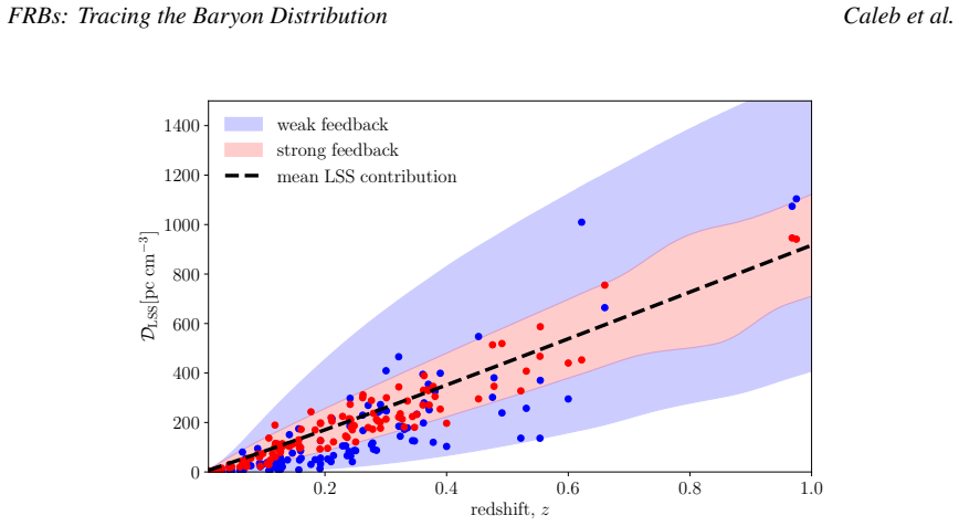
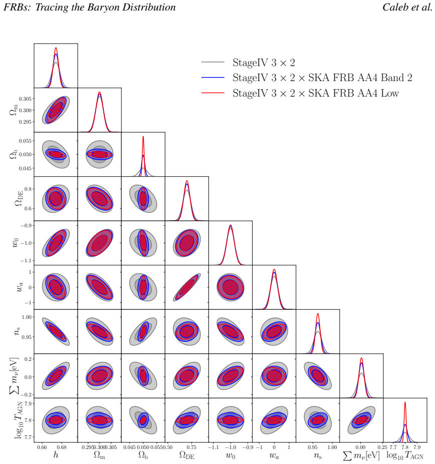
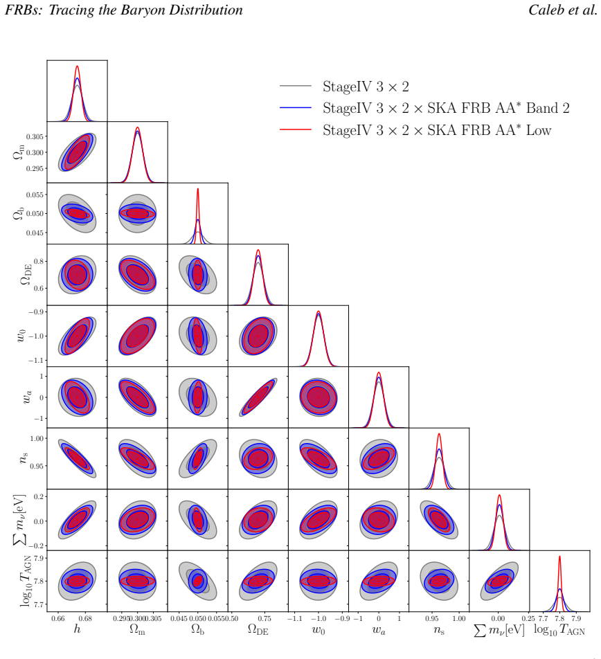
Forecasts demonstrate that SKA detections of fast radio bursts will measure the redshift-dependent scatter in dispersion measure, the statistical properties of the dispersion-measure field, and its cross-correlation with cosmic shear and galaxy clustering from Stage IV surveys, thereby distinguishing baryonic feedback scenarios and recovering cosmological information otherwise masked by astrophysical effects; the same observations will additionally constrain circumgalactic-medium properties via scattering timescales and improve constraints on the epoch of reionisation.
What carries the argument
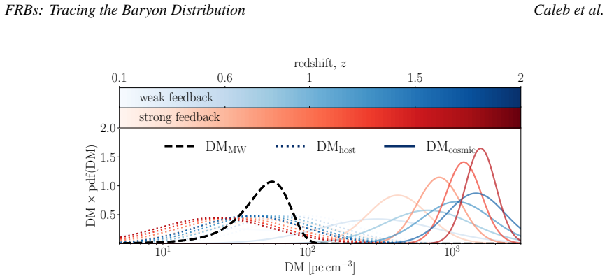
Dispersion measure (DM) of fast radio bursts, which integrates the line-of-sight ionized electron density and serves as a direct baryon tracer.
If this is right
- Baryonic feedback models can be pinpointed, recovering cosmological signals masked in Stage IV galaxy surveys.
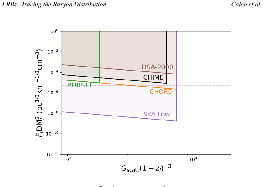
- Circumgalactic medium properties can be measured directly from FRB scattering timescales.
- The large redshift range of SKA FRBs improves constraints on the epoch of reionisation.
- The mechanism behind fast radio bursts may be clarified by the extended redshift coverage.
Where Pith is reading between the lines
- If feedback models are better pinned down, derived parameters such as the sum of neutrino masses from weak-lensing surveys would shift by amounts comparable to current statistical uncertainties.
- The same DM field maps could be cross-checked against X-ray or Sunyaev-Zeldovich observations of the warm-hot intergalactic medium to test consistency of the ionized fraction.
- A mismatch between predicted and observed DM cross-spectra would indicate either missing feedback physics or an unaccounted systematic in the FRB host-galaxy contribution.
Load-bearing premise
The statistical properties of the dispersion-measure field, including scatter versus redshift and cross-power spectra, can be modeled from existing data and simulations with enough accuracy to separate feedback models once SKA statistics arrive.
What would settle it
If the measured DM scatter versus redshift and cross-power spectra with galaxy surveys from the first few years of SKA data do not separate the feedback models that current simulations predict to be distinguishable, the claimed improvement in cosmological constraining power does not occur.
Figures
read the original abstract
Baryonic feedback redistributes matter on small to mid cosmological scales, ultimately limiting inferences from Stage IV galaxy surveys. Direct baryon tracers are crucial for recovering cosmological signals masked by astrophysical effects, and vice versa: galaxy formation and other astrophysical processes must be interpreted cosmologically. Fast radio bursts (FRBs) serve as such tracers: their dispersion measure (DM) records the line-of-sight integrated ionised electron density. The Square Kilometre Array (SKA) will be the only radio telescope capable of detecting many FRBs in the southern hemisphere, significantly enhancing synergy with surveys such as Rubin Observatory. This chapter completes the FRB trilogy by forecasting the SKA's potential to constrain the baryon distribution from cosmological to galactic scales and across cosmic time. We tackle this question by investigating the DM scatter as a function of redshift. We also study the statistical properties of the DM field and its cross-correlation with Stage IV galaxy surveys. Our focus is on cosmic shear and galaxy clustering. This shows that the SKA can play a crucial role in pinpointing baryonic feedback models, thereby greatly enhancing the cosmological constraining power of Stage IV galaxy surveys. Furthermore, we show that the SKA will be able to measure the properties of the circumgalactic medium using the scattering timescale of FRBs. Lastly, the large redshift range of FRB detections with the SKA can improve our understanding of the epoch of reionisation. It may also clarify the mechanism behind FRBs.
Editorial analysis
A structured set of objections, weighed in public.
Referee Report
Summary. The manuscript forecasts the potential of Fast Radio Bursts (FRBs) detected by the Square Kilometre Array (SKA) to constrain the baryon distribution from cosmological to galactic scales. It focuses on the redshift dependence of dispersion measure (DM) scatter, the statistical properties of the DM field, and cross-correlations of the DM field with cosmic shear and galaxy clustering from Stage IV surveys. The central claim is that these measurements will pinpoint baryonic feedback models and thereby enhance the cosmological constraining power of Stage IV galaxy surveys; additional forecasts address the circumgalactic medium via scattering timescales and the epoch of reionization.
Significance. If the modeling assumptions hold, the work would be significant for planning multi-tracer cosmological analyses, as it quantifies how radio FRB data can mitigate baryonic uncertainties that limit optical Stage IV surveys. The emphasis on cross-correlations and redshift evolution provides concrete projections that could inform survey strategy. The paper does not include machine-checked proofs or parameter-free derivations, but the forecasts are presented as falsifiable once SKA data arrive.
major comments (2)
- [Abstract; DM field statistics section] The forecasts for distinguishing baryonic feedback models via DM scatter versus redshift and DM cross-power spectra with cosmic shear/galaxy clustering (Abstract and the section on statistical properties of the DM field) rest on the assumption that these quantities can be forward-modeled from existing FRB catalogs and simulations with sufficient fidelity. No quantitative validation or error propagation from sub-grid feedback uncertainties is shown, which directly affects the claimed enhancement of Stage IV constraints.
- [Cross-correlation forecasts section] The claim that SKA FRBs will 'greatly enhance' cosmological constraining power (Abstract) requires explicit demonstration that mismatches between assumed and true DM scatter or cross-spectra would not degrade the forecasted gains; the manuscript provides no such sensitivity test.
minor comments (2)
- [Methods/forecast setup] Clarify the exact redshift range and number of FRBs assumed for the SKA forecasts, as these choices affect all quantitative projections.
- [CGM section] The discussion of scattering timescales for the circumgalactic medium would benefit from a brief comparison to existing FRB scattering measurements to anchor the projections.
Simulated Author's Rebuttal
We thank the referee for their constructive comments on our forecasting study. We address the two major comments point by point below and will revise the manuscript to incorporate additional discussion of modeling uncertainties and sensitivity tests.
read point-by-point responses
-
Referee: [Abstract; DM field statistics section] The forecasts for distinguishing baryonic feedback models via DM scatter versus redshift and DM cross-power spectra with cosmic shear/galaxy clustering (Abstract and the section on statistical properties of the DM field) rest on the assumption that these quantities can be forward-modeled from existing FRB catalogs and simulations with sufficient fidelity. No quantitative validation or error propagation from sub-grid feedback uncertainties is shown, which directly affects the claimed enhancement of Stage IV constraints.
Authors: We agree that the manuscript would benefit from explicit discussion of how sub-grid feedback uncertainties propagate into the forecasted DM statistics. Our forecasts are derived from DM fields extracted from a suite of hydrodynamical simulations that include baryonic feedback, but we did not perform a systematic variation across different sub-grid prescriptions or propagate those variations into the final constraints. In the revised version we will add a dedicated subsection that quantifies the impact of simulation-to-simulation differences on the redshift-dependent DM scatter and on the DM–shear and DM–galaxy cross-spectra, including a simple error-propagation estimate. This will directly support (or qualify) the claimed enhancement of Stage IV cosmological constraints. revision: yes
-
Referee: [Cross-correlation forecasts section] The claim that SKA FRBs will 'greatly enhance' cosmological constraining power (Abstract) requires explicit demonstration that mismatches between assumed and true DM scatter or cross-spectra would not degrade the forecasted gains; the manuscript provides no such sensitivity test.
Authors: The statement that SKA FRBs will 'greatly enhance' cosmological power is based on the nominal forecasts. We acknowledge that the manuscript does not contain a sensitivity analysis exploring how deviations between the assumed and true DM scatter or cross-spectra would affect the final gains. In the revised manuscript we will add a short sensitivity study in which we vary the input DM scatter and cross-power amplitudes within ranges consistent with current simulation uncertainties and recompute the improvement in cosmological parameter constraints. This will provide the explicit robustness check requested. revision: yes
Circularity Check
No significant circularity in forecasting approach
full rationale
The paper presents forecasts for SKA constraints on baryonic feedback using external models of the DM field, FRB populations, and simulations. The central claims about enhancing Stage IV cosmological power rest on forward-modeling assumptions for DM scatter and cross-spectra that are not derived from or equivalent to the paper's own results by construction. No equations or self-citations reduce the predictions to fitted inputs, and the methodology is self-contained against external benchmarks without self-definitional loops or load-bearing self-citations.
Axiom & Free-Parameter Ledger
Reference graph
Works this paper leans on
-
[1]
doi: 10.1051/0004-6361/201526328. S. Amodeo et al.PRD, 103(6):063514, Mar
-
[2]
doi: 10.1103/PhysRevD.103.063514. M. Ayromlou, D. Nelson, and A. Pillepich.MNRAS, 524(4):5391–5410, Oct
-
[3]
doi: 10.1093/mnras/stab309. M. Bhattacharya, P. Kumar, and E. V. Linder.PRD, 103(10):103526, May
-
[4]
doi: 10.1093/mnras/stae2100. V. Bonjean et al.A&A, 609:A49, Jan
-
[5]
doi: 10.1051/0004-6361/201731699. J. N. Bregman.ARA&A, 45(1):221–259, Sept
-
[6]
doi: 10.1146/annurev.astro.45.051806. 110619. 19 FRBs: Tracing the Baryon Distribution Caleb et al. J. N. Bregman et al.ApJ, 699(2):1765–1774, July
-
[7]
doi: 10.1088/0004-637X/699/2/1765. M. Caleb et al.MNRAS, 524(2):2064–2077, 06
-
[9]
CHIME/FRB Collaboration et al.ApJS, 257(2):59, December
doi: 10.3847/1538-4365/ac6fd9. CHIME/FRB Collaboration et al.ApJS, 257(2):59, December
-
[10]
doi: 10.3847/1538-4365/ ac33ab. N. E. Chisari et al.OJA, 2(1):4, June
-
[11]
doi: 10.21105/astro.1905.06082. L. Connor et al.Nature Astronomy, June
work page internal anchor Pith review Pith/arXiv arXiv doi:10.21105/astro.1905.06082 1905
-
[12]
doi: 10.1038/s41550-025-02566-y. R. J. Cooke, M. Pettini, and C. C. Steidel.ApJ, 855(2):102, Mar
-
[13]
doi: 10.3847/1538-4357/ aaab53. K. Cranmer, J. Brehmer, and G. Louppe.Proceedings of the National Academy of Science, 117 (48):30055–30062, Dec
-
[14]
doi: 10.1073/pnas.1912789117. A. P. Curtin et al. InAdvancing Astrophysics with the SKA – II (AASKAII)
-
[15]
doi: 10.1103/RevModPhys.88.015004. J.-P. Dai and J.-Q. Xia.MNRAS, 503(3):4576–4580, May
-
[16]
S.Das,Y.-K.Chiang,andS.Mathur.ApJ,951(2):125,July2023
doi: 10.1093/mnras/stab785. S.Das,Y.-K.Chiang,andS.Mathur.ApJ,951(2):125,July2023. doi: 10.3847/1538-4357/acd764. A. de Graaff, Y.-C. Cai, C. Heymans, and J. A. Peacock.A&A, 624:A48, Apr
-
[17]
doi: 10.1051/0004-6361/201935159. D. Eckert et al.nat, 528(7580):105–107, Dec
-
[18]
Euclid Collaboration et al.A&A, 642:A191, Oct
doi: 10.1038/nature16058. Euclid Collaboration et al.A&A, 642:A191, Oct
-
[19]
doi: 10.1051/0004-6361/202038071. C.-A. Faucher-Giguère and S. P. Oh.ARA&A, 61:131–195, Aug
-
[20]
A Fast Radio Burst Occurs Every Second throughout the Observable Universe
ISSN 2041-8205, 2041-8213. doi: 10.3847/2041-8213/aa8905. arXiv:1706.06582 [astro-ph]. M. Fukugita and P. J. E. Peebles.ApJ, 616(2):643–668, Dec
work page internal anchor Pith review Pith/arXiv arXiv doi:10.3847/2041-8213/aa8905 2041
-
[21]
doi: 10.1086/425155. S. Grandis, G. Aricò, A. Schneider, and L. Linke.MNRAS, 528(3):4379–4392, Mar
-
[22]
20 FRBs: Tracing the Baryon Distribution Caleb et al
doi: 10.1093/mnras/stae259. 20 FRBs: Tracing the Baryon Distribution Caleb et al. B. Hadzhiyska et al.arXiv e-prints, art. arXiv:2407.07152, July
-
[23]
doi: 10.48550/arXiv.2407. 07152. S.Hagstotz,R.Reischke,andR.Lilow.MNRAS,511(1):662–667,Mar.2022. doi: 10.1093/mnras/ stac077. N. Hand et al.PRL, 109(4):041101, July
-
[24]
doi: 10.1103/PhysRevLett.109.041101. S. Heimersheim, N. S. Sartorio, A. Fialkov, and D. R. Lorimer.ApJ, 933(1):57, July
-
[25]
doi: 10.3847/1538-4357/ac70c9. A. W. Hotan et al.PASA, 38:e009, March
-
[26]
doi: 10.1017/pasa.2021.1. T.-Y. Hsu et al.A&A, 698:A163, June
-
[27]
doi: 10.1051/0004-6361/202452714. M. Hussaini et al.arXiv e-prints, art. arXiv:2506.04186, June
-
[28]
doi: 10.48550/arXiv.2506. 04186. C. W. James et al.MNRAS, 516(4):4862–4881, Nov
-
[29]
doi: 10.1093/mnras/stac2524. M. Jaroszynski.MNRAS, 484(2):1637–1644, Apr
-
[30]
ISSN 0035-8711, 1365-2966. doi: 10.1093/mnras/sty3529. D. L. Jow, X. Wu, and U.-L. Pen.PNAS, 121(39):e2406783121, Sept
-
[31]
doi: 10.1073/pnas. 2406783121. K. I. Kellermann and I. I. K. Pauliny-Toth.ApJL, 155:L71, Feb
-
[32]
doi: 10.1086/180305. I. S. Khrykin et al.ApJ, 973(2):151, Oct
-
[33]
doi: 10.3847/1538-4357/ad6567. K. Konar et al.OJA, 8:102, July
-
[34]
doi: 10.33232/001c.142524. R. M. Konietzka et al.arXiv e-prints, art. arXiv:2507.07090, July
-
[35]
Kovač et al.arXiv e-prints, art
M. Kovač et al.arXiv e-prints, art. arXiv:2507.07991, July
-
[36]
doi: 10.3847/1538-4357/ad3736. C.Leungetal.arXive-prints,art.arXiv:2509.19514,Sept.2025. doi: 10.48550/arXiv.2509.19514. Z. Li et al.ApJ, 876(2):146, May
-
[37]
doi: 10.3847/1538-4357/ab18fe. M.LoVerdeandN.Afshordi.PRD,78(12):123506,Dec.2008.doi: 10.1103/PhysRevD.78.123506. J. P. Macquart et al. InAdvancing Astrophysics with the Square Kilometre Array (AASKA14), page 55, Apr
-
[38]
doi: 10.22323/1.215.0055. J. P. Macquart et al.nat, 581(7809):391–395, May
-
[39]
doi: 10.1038/s41586-020-2300-2. B. Maity.A&A, 689:A340, Sept
-
[40]
K.W.MasuiandK.Sigurdson.PRL,115(12):121301,Sept.2015
doi: 10.1051/0004-6361/202451160. K.W.MasuiandK.Sigurdson.PRL,115(12):121301,Sept.2015. doi: 10.1103/PhysRevLett.115. 121301. I. G. McCarthy et al.MNRAS, 540(1):143–163, June
-
[41]
21 FRBs: Tracing the Baryon Distribution Caleb et al
doi: 10.1093/mnras/staf731. 21 FRBs: Tracing the Baryon Distribution Caleb et al. M. McCourt, S. P. Oh, R. O’Leary, and A.-M. Madigan.MNRAS, 473(4):5407–5431, Feb
-
[42]
doi: 10.1093/mnras/stx2687. M. McQuinn.ApJL, 780(2):L33, Jan
-
[43]
doi: 10.1088/2041-8205/780/2/L33. M. McQuinn.ARA&A, 54:313–362, Sept
work page internal anchor Pith review doi:10.1088/2041-8205/780/2/l33 2041
-
[44]
doi: 10.1146/annurev-astro-082214-122355. I. Medlock, D. Nagai, D. Anglés-Alcázar, and M. Gebhardt.ApJ, 983(1):46, Apr. 2025a. doi: 10.3847/1538-4357/adbc9c. I. Medlock et al.ApJ, 980(1):61, Feb. 2025b. doi: 10.3847/1538-4357/ada442. F. Nicastro et al.NAT, 558(7710):406–409, June
-
[45]
doi: 10.1038/s41586-018-0204-1. S. K. Ocker, J. M. Cordes, S. Chatterjee, and M. R. Gorsuch.ApJ, 934(1):71, July
-
[46]
doi: 10.3847/1538-4357/ac75ba. S. K. Ocker, M. C. Chen, S. P. Oh, and P. Sharma.ApJ, 988(1):69, July
-
[48]
doi: 10.48550/ arXiv.1605.06376. S. V. Penton, J. T. Stocke, and J. M. Shull.ApJS, 152(1):29–62, May
work page internal anchor Pith review Pith/arXiv arXiv
-
[49]
Planck Collaboration et al.A&A, 641:A6, Sept
doi: 10.1086/382877. Planck Collaboration et al.A&A, 641:A6, Sept
-
[50]
doi: 10.1051/0004-6361/201833910. M. Rafiei-Ravandi et al.ApJ, 922(1):42, Nov
-
[51]
doi: 10.3847/1538-4357/ac1dab. K. M. Rajwade et al.MNRAS, 514(2):1961–1974, Aug
-
[52]
doi: 10.1093/mnras/stac1450. R. Reischke and S. Hagstotz.MNRAS, 524:2237–2243, Sept
-
[53]
A first measurement of baryonic feedback with Fast Radio Bursts
ISSN 0035-8711. doi: 10.1093/mnras/stad1645. R. Reischke and S. Hagstotz.arXiv e-prints, art. arXiv:2507.17742, July
work page internal anchor Pith review Pith/arXiv arXiv doi:10.1093/mnras/stad1645
-
[54]
doi: 10.48550/ arXiv.2507.17742. R. Reischke, S. Hagstotz, and R. Lilow.PRD, 103(2):023517, Jan
work page internal anchor Pith review Pith/arXiv arXiv
-
[55]
doi: 10.1103/PhysRevD. 103.023517. R. Reischke et al.OJA, 8:127, Sept
-
[56]
R.Reischkeetal.J.CosmologyAstropart.Phys.,2026(6):006,June2026.doi: 10.1088/1475-7516/ 2026/06/006
doi: 10.33232/001c.143819. R.Reischkeetal.J.CosmologyAstropart.Phys.,2026(6):006,June2026.doi: 10.1088/1475-7516/ 2026/06/006. D.H.Rudd,A.R.Zentner,andA.V.Kravtsov.ApJ,672(1):19–32,Jan.2008.doi: 10.1086/523836. G. C. Rudie et al.ApJ, 885(1):61, Nov
-
[57]
doi: 10.3847/1538-4357/ab4255. E. Schaan et al.PRD, 93(8):082002, Apr
-
[58]
doi: 10.1103/PhysRevD.93.082002. E. Schaan et al.PRD, 103(6):063513, Mar
-
[59]
doi: 10.1103/PhysRevD.103.063513. J. Schaye et al.MNRAS, 526(4):4978–5020, Dec
-
[60]
22 FRBs: Tracing the Baryon Distribution Caleb et al
doi: 10.1093/mnras/stad2419. 22 FRBs: Tracing the Baryon Distribution Caleb et al. A. Schneider, S. K. Giri, S. Amodeo, and A. Refregier.MNRAS, 514(3):3802–3814, Aug
-
[61]
E.Sembolonietal.MNRAS,417(3):2020–2035,Nov.2011
doi: 10.1093/mnras/stac1493. E.Sembolonietal.MNRAS,417(3):2020–2035,Nov.2011. doi: 10.1111/j.1365-2966.2011.19385. x. R.M.Shannonetal.arXive-prints,art.arXiv:2408.02083,Aug.2024. doi: 10.48550/arXiv.2408. 02083. K. Sharma et al.ApJ, 989(1):81, Aug
-
[62]
doi: 10.3847/1538-4357/adeca4. K. Sharma et al.ApJ, 998(1):109, Feb
-
[63]
doi: 10.3847/1538-4357/ae2ff9. J.M.Shull,B.D.Smith,andC.W.Danforth.ApJ,759(1):23,Nov.2012. doi: 10.1088/0004-637X/ 759/1/23. J.Siegeletal.arXive-prints,art.arXiv:2512.02954,Dec.2025. doi: 10.48550/arXiv.2512.02954. B. Soergel et al.MNRAS, 461(3):3172–3193, Sept
work page internal anchor Pith review Pith/arXiv arXiv doi:10.3847/1538-4357/ae2ff9 2012
-
[64]
doi: 10.1093/mnras/stw1455. R. Takahashi, K. Ioka, A. Mori, and K. Funahashi.MNRAS, 502(2):2615–2629, Apr
-
[65]
doi: 10.1093/mnras/stab170. H. Tanimura et al.A&A, 637:A41, May 2020a. doi: 10.1051/0004-6361/201937158. H. Tanimura et al.A&A, 643:L2, Nov. 2020b. doi: 10.1051/0004-6361/202038521. N. Tessore et al.OJA, 6:11, Mar
-
[66]
The Open Journal of Astrophysics , keywords =
doi: 10.21105/astro.2302.01942. A.Theis,S.Hagstotz,R.Reischke,andJ.Weller.arXive-prints,art.arXiv:2403.08611,Mar.2024. doi: 10.48550/arXiv.2403.08611. M. Torkamani et al.arXiv e-prints, art. arXiv:2601.18784, Jan
-
[67]
doi: 10.48550/arXiv.2601. 18784. T. Tröster et al.A&A, 660:A27, Apr
-
[68]
doi: 10.1051/0004-6361/202142197. O. Tsang and J. G. Kirk.A&A, 463(1):145–152, Feb
-
[69]
doi: 10.1051/0004-6361:20066502. J. Tumlinson, M. S. Peeples, and J. K. Werk.ARA&A, 55(1):389–432, Aug
-
[70]
doi: 10.1111/j.me1365-2966.2011.18981.x. M. P. van Daalen, I. G. McCarthy, and J. Schaye.MNRAS, 491(2):2424–2446, Jan
-
[71]
doi: 10.1093/mnras/stz3199. H. K. Vedantham and E. S. Phinney.MNRAS, 483(1):971–984, Feb
-
[72]
doi: 10.1093/mnras/ sty2948. C. R. H. Walker et al.A&A, 683:A71, Mar
-
[73]
doi: 10.1051/0004-6361/202347139. A. Walters et al.ApJ, 856(1):65, Mar
-
[74]
23 FRBs: Tracing the Baryon Distribution Caleb et al
doi: 10.3847/1538-4357/aaaf6b. 23 FRBs: Tracing the Baryon Distribution Caleb et al. A. Walters, Y.-Z. Ma, J. Sievers, and A. Weltman.PRD, 100(10):103519, Nov
-
[75]
doi: 10.1103/PhysRevD.100.103519. B. Wang and J.-J. Wei.ApJ, 944(1):50, Feb
-
[76]
doi: 10.3847/1538-4357/acb2c8. A. Wayland, D. Alonso, and R. Reischke.arXiv e-prints, art. arXiv:2602.12174, Feb
work page internal anchor Pith review Pith/arXiv arXiv doi:10.3847/1538-4357/acb2c8
-
[77]
doi: 10.48550/arXiv.2602.12174. Y. Zhang et al.A&A, 690:A268, Oct
work page internal anchor Pith review Pith/arXiv arXiv doi:10.48550/arxiv.2602.12174
-
[78]
doi: 10.1051/0004-6361/202449413. Z. J. Zhang et al.ApJ, 906(1):49, Jan
-
[79]
doi: 10.3847/1538-4357/abceb9. 24
discussion (0)
Sign in with ORCID, Apple, or X to comment. Anyone can read and Pith papers without signing in.