REVIEW 5 major objections 4 minor 38 references
D3FL: Data Distribution and Detrending for Robust Federated Learning in Non-linear Time-series Data
T0 review · 5 major / 4 minor · reviewed 2026-08-06 · deepseek-v4-flash
Pith's one-line read The paper claims that federated learning with FedAvg is less accurate than centralized training on non-linear time series, and that the right detrending method closes much of that gap.
desk verdict A useful but under-specified benchmark; the detrending claims hinge on an unstated fit-before-split choice that risks lookahead leakage. read the letter →
The pith
A machine-rendered reading of the paper's core claim, the machinery that carries it, and where it could break.
The reading
What carries the argument
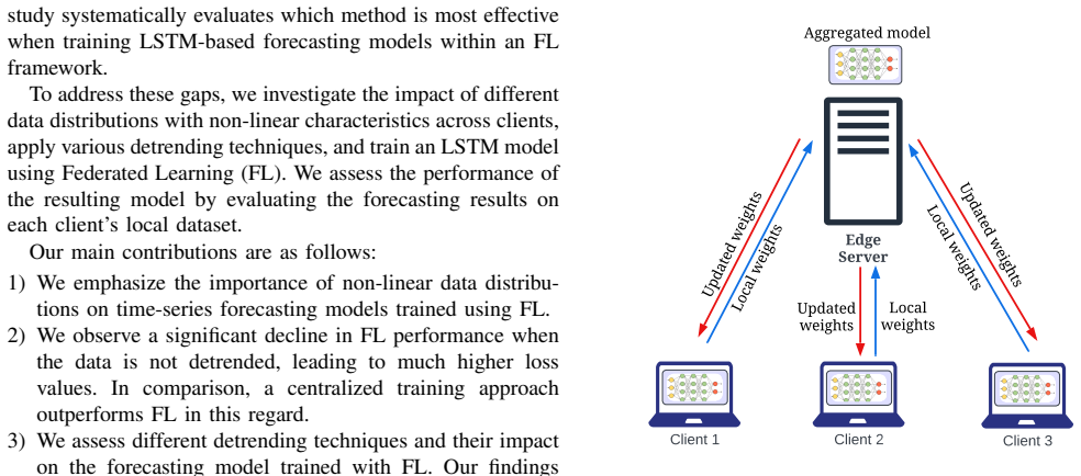
The carrying protocol is a ten-client comparison between centralized training and FedAvg, using a one-layer LSTM (24-step input, 2-step output) as the shared forecaster. Each client holds a univariate series drawn from either the generalized extreme value (GEV) or log-normal family, with parameters chosen so values fall roughly in a 2-to-20 range. The manipulation is detrending, applied before the chronological 90/10 train/validation split, using five standard techniques: first differencing, sliding-window moving average removal, mean removal, linear regression subtraction, and quadratic regression subtraction. These methods convert each non-stationary series into a near-stationary residual series; the paper's finding is that the optimal conversion depends on the underlying distribution.
What would settle it
Re-run the synthetic and real-world experiments with all detrending statistics computed inside the training window only, using a walk-forward or expanding-window estimation, and compare the validation MSE values against Tables IV-VII; if the detrending advantage largely disappears, the reported gains were lookahead artifacts.
Extended reading notes
Core claim
On its own terms, the paper's central discovery is that non-linear, non-stationary client data distributions degrade the performance of a standard FedAvg-LSTM forecaster, and that an appropriate detrending step recovers most of the loss. Without detrending, FL validation MSE on synthetic gen-extreme data was 0.00844 versus 0.00273 for centralized training, and the log-normal case rose from 0.00589 to 0.01583; mixing both distributions widened the FL gap further. With detrending, FL MSE fell to 0.00554 for gen-extreme (differencing) and 0.01339 for log-normal (differencing) on synthetic data, while on the real-world Ausgrid data the lowest FL losses came from quadratic detrending for gen-extreme and mean subtraction for log-normal. The paper reads these results as evidence that the choice of detrending method is distribution-dependent and that detrending should be part of the FL pipeline.
Load-bearing premise
The experiments assume that detrending statistics (moving average, mean, and regression coefficients) are computed without looking at the validation portion of each time series, but the paper never states that they are estimated on the training portion only.
Editorial extensions
If this is right
- FL practitioners should expect a non-linear or heavy-tailed client distribution to widen the gap between federated and centralized forecast error, independent of communication constraints.
- Detrending is not neutral in FL: the wrong method can raise validation loss, so the choice should be matched to the client data distribution.
- On synthetic series, first-order differencing gave the lowest federated validation error for both GEV and log-normal clients, suggesting residual-based training helps the global model.
- The mixed-distribution experiment implies that the presence of log-normal clients disproportionately raises the global FedAvg validation loss, which may inform client selection.
Reading between the lines
- If the detrending gains survive a strictly causal re-run, a natural extension is per-client detrending choice communicated as metadata to the server, which could beat any single global method.
- The disagreement between the synthetic result (differencing best) and the real-world result (quadratic or mean removal best) suggests the optimal method depends on trend shape and noise, not just the marginal distribution; a testable hypothesis is that differencing wins for stochastic trends and polynomial removal for smooth deterministic trends.
- A mechanism the authors leave implicit is that detrending makes clients' residual series more alike, reducing FedAvg gradient conflict; measuring client-weight divergence before and after detrending would test this directly.
- Because the paper does not specify when detrending statistics are computed, its FL-versus-centralized comparison should be re-run under strictly causal preprocessing before the specific loss numbers are used for design decisions.
Signed reviews
Editorial analysis
A structured set of objections, weighed in public.
Referee Report
Summary. The paper studies how non-linear, non-stationary time-series distributions (generalized extreme value, log-normal, and a mix) affect LSTM forecasting under FedAvg versus centralized training, and evaluates five detrending techniques. Experiments on synthetic data and Ausgrid substation data report validation MSE, RMSE, and MAE; the central claims are that FL underperforms centralized training on such data and that choosing an appropriate detrending method reduces forecasting loss across distributions.
Significance. If confirmed, the comparison provides useful empirical evidence for practitioners choosing between FL and centralized training for non-linear IoT time-series forecasting, and it highlights that the detrending choice matters in FL. The use of controlled synthetic data with known distribution families is a strength, as is the inclusion of a real-world energy dataset and the systematic comparison of six preprocessing settings. The paper does not introduce theory or release code, so its contribution is primarily empirical; however, the current experimental reporting lacks repeated runs, a held-out test set, and precise preprocessing details, which limits the strength of the stated claims.
major comments (5)
- [§IV-A and §II-C (Eqs. 5–7)] The manuscript never states whether detrending statistics are estimated on each client's training prefix or on the full series before the 90/10 chronological split. Equations (5)–(7) define the mean, linear, and quadratic coefficients over the whole series, and Section IV-A only describes the split for training and validation data. If the full series is used, the validation segment contributes to the transform, so the detrending gains in Tables V and VII could be lookahead artifacts rather than genuine forecasting improvements. Please clarify the fitting window; if the full series was used, re-run the experiments with the statistics computed on the training portion only.
- [Tables IV–VII] All results are reported as single point estimates with no indication of random seeds, number of runs, or error bars. For example, in Table V the FL gen-extreme MSE for differencing is 0.00554 versus 0.00677 for moving average; without variance information it is impossible to tell whether this difference is meaningful. Because the paper's second contribution is a recommendation to select an "appropriate" detrending method from exactly these numbers, the absence of repeated runs is load-bearing. Please report means and standard deviations over multiple seeds and, where possible, a significance test.
- [§VI.B.2 and Tables VI–VII] No held-out test set is used: the validation split described in Section IV-A serves both to select the best detrending method and to report final performance. For instance, the claim that quadratic detrending "yielded the best results" on Ausgrid gen-extreme data is based on the same validation losses in Table VII that were used for method selection. This double use can overstate the benefit of the chosen method. Please add a held-out test segment after model selection and report performance on that segment.
- [Table VII] The centralized RMSE values are internally inconsistent with the reported MSE values for gen-extreme data. For the moving-average row, MSE = 0.0000011 but RMSE = 0.0077, whereas the square root of the MSE is approximately 0.00105; similar mismatches appear for the linear (MSE = 0.0000068, RMSE = 0.0072) and quadratic (MSE = 0.0000098, RMSE = 0.0074) rows. Since Table VII is the basis for the real-world detrending conclusions, these inconsistencies must be corrected or the affected conclusions revisited.
- [§II-C and §IV-B] Several parameters required to reproduce the experiments are not reported. Equation (4) defines a moving average with a window of size p, but no value of p is given anywhere; Section IV-B describes the synthetic data generation only qualitatively ("a sine function", "an additional offset") without the exact formulas or parameter values; and Section IV-D mentions a grid search over lookback and lookahead but not the search ranges. These omissions are material because the moving-average and synthetic-data results are central to the paper's conclusions.
minor comments (4)
- [Eq. (4)] The denominator in the moving-average formula is written as n but the sum runs over p terms; the notation should be made consistent, with p defined.
- [Figure 9] The fourth panel in the log-normal figure is labeled "Subtracting mean" twice; the second occurrence should be "Linear model" to match the other figures.
- [Section V and Section VI.A.2] The experiment count is stated inconsistently: Section V says eighteen experiments on each dataset, while Section VI.A.2 says 15 detrending experiments and 30 total experiments per setup; please clarify the counting.
- [Throughout] The paper alternates between "log norm" and "log normal"; standardize the terminology, especially in the abstract and tables.
Circularity Check
No circularity found: both headline claims are direct empirical benchmarks against synthetic and real time-series data, and the only self-citation concerns the experimental harness, not the scientific conclusions.
full rationale
The paper's central claims are empirical comparisons, not derivations. 'FL performs worse than centralized approaches when dealing with non-linear data distributions' and 'the use of appropriate detrending techniques improves FL performance, reducing loss across different data distributions' are supported by direct loss comparisons in Tables IV-VII against GEV and log-normal synthetic series and the Ausgrid dataset. No parameter is fitted to a subset and then reported as a prediction of a closely related quantity; no uniqueness theorem or prior theoretical result by these authors is invoked to force a conclusion. The only self-citation, 'The Flotilla framework [35] has been used for running FL on edge devices and Docker containers', concerns the experimental infrastructure and is not load-bearing for either headline claim. The post-hoc identification of empirically better detrending methods, such as 'the differencing technique proved to be the most effective' and 'quadratic detrending yielded the best results', is a descriptive experimental finding rather than a self-definitional reduction: 'appropriate' is not formally defined as 'the method that wins in the same validation table', though a pre-registered or held-out method-selection rule would strengthen the generalization. The possible use of full-series detrending statistics in Equations 5-7 before the 90/10 chronological split would be a data-leakage or correctness concern, not circularity, because it does not make any equation identical to its own input by construction. Therefore no specific circular step can be quoted and no circularity score above 0 is warranted.
Assumptions & free parameters
free parameters (3)
- Synthetic GEV and log-normal distribution parameters =
Not reported; chosen so data values fall in range 2 to 20
- Moving-average window size p =
Not reported
- LSTM lookback and lookahead =
24 input steps, 2 output steps
assumptions (5)
- domain assumption Extreme weather and temperature data follow a generalized extreme value distribution, and financial data follow log-normal or log-gamma distributions.
- domain assumption Detrending to remove trends and seasonality improves forecasting model performance.
- domain assumption FedAvg with one local epoch per global round is a representative FL setup for the conclusions.
- domain assumption Ideal network conditions do not affect the model-performance comparison.
- domain assumption The 10 selected Ausgrid substations genuinely follow the assigned GEV or log-normal distributions.
Cite this review
Pith. "Pith review of D3FL: Data Distribution and Detrending for Robust Federated Learning in Non-linear Time-series Data." pith.science (2026). https://pith.science/paper/LLLXPTEQ
@misc{pith2026250711471,
  author       = {Pith},
  title        = {Pith review of: D3FL: Data Distribution and Detrending for Robust Federated Learning in Non-linear Time-series Data},
  year         = {2026},
  howpublished = {\url{https://pith.science/paper/LLLXPTEQ}},
  note         = {Machine review of arXiv:2507.11471}
}
read the original abstract
With advancements in computing and communication technologies, the Internet of Things (IoT) has seen significant growth. IoT devices typically collect data from various sensors, such as temperature, humidity, and energy meters. Much of this data is temporal in nature. Traditionally, data from IoT devices is centralized for analysis, but this approach introduces delays and increased communication costs. Federated learning (FL) has emerged as an effective alternative, allowing for model training across distributed devices without the need to centralize data. In many applications, such as smart home energy and environmental monitoring, the data collected by IoT devices across different locations can exhibit significant variation in trends and seasonal patterns. Accurately forecasting such non-stationary, non-linear time-series data is crucial for applications like energy consumption estimation and weather forecasting. However, these data variations can severely impact prediction accuracy. The key contributions of this paper are: (1) Investigating how non-linear, non-stationary time-series data distributions, like generalized extreme value (gen-extreme) and log norm distributions, affect FL performance. (2) Analyzing how different detrending techniques for non-linear time-series data influence the forecasting model's performance in a FL setup. We generated several synthetic time-series datasets using non-linear data distributions and trained an LSTM-based forecasting model using both centralized and FL approaches. Additionally, we evaluated the impact of detrending on real-world datasets with non-linear time-series data distributions. Our experimental results show that: (1) FL performs worse than centralized approaches when dealing with non-linear data distributions. (2) The use of appropriate detrending techniques improves FL performance, reducing loss across different data distributions.
Figures


Figures from the paper (9 more)





Reference graph
Works this paper leans on
-
[1]
Iot connections worldwide 2022-2033
Lionel Sujay Vailshery. Iot connections worldwide 2022-2033. https:// www.statista.com/statistics/1183457/iot-connected-devices-worldwide/,
arXiv 2022
-
[2]
Dawei Zhang. A yolo-based approach for fire and smoke detection in iot surveillance systems.International Journal of Advanced Computer Science & Applications, 15(1), 2024
work page 2024
-
[3]
Hongyan Dui, Songru Zhang, Meng Liu, Xinghui Dong, and Guanghan Bai. Iot-enabled real-time traffic monitoring and control management for intelligent transportation systems.IEEE Internet of Things Journal, 2024
work page 2024
-
[4]
Montaser NA Ramadan, Mohammed AH Ali, Shin Yee Khoo, Moham- mad Alkhedher, and Mohammad Alherbawi. Real-time iot-powered ai system for monitoring and forecasting of air pollution in industrial environment.Ecotoxicology and Environmental Safety, 283:116856, 2024
work page 2024
-
[5]
Internet of things (iot) based energy monitoring with esp 32 and using thingspeak
Mareddy Anusha, Pavuluri Bhavan Kumar, Vangari Akhil, Matam Gouthami, MC Chinnaaiah, and Shafi Shaik. Internet of things (iot) based energy monitoring with esp 32 and using thingspeak. In2024 10th International Conference on Communication and Signal Processing (ICCSP), pages 1383–1387. IEEE, 2024
work page 2024
-
[6]
Electrical load forecasting using edge computing and federated learning
Afaf Ta ¨ık and Soumaya Cherkaoui. Electrical load forecasting using edge computing and federated learning. InICC 2020-2020 IEEE international conference on communications (ICC), pages 1–6. IEEE, 2020
work page 2020
-
[7]
Feng Xie, Sebastian Naumann, Olaf Czogalla, and Hartmut Zadek. Machine learning model application and comparison in actuated traffic signal forecasting.Sensors, 23(15):6912, 2023
work page 2023
-
[8]
A meta-graph deep learning framework for forecasting air pollutants in stockholm
Zhiguo Zhang, Xiaoliang Ma, Christer Johansson, Junchen Jin, and Magnuz Engardt. A meta-graph deep learning framework for forecasting air pollutants in stockholm. In2023 IEEE 9th World Forum on Internet of Things (WF-IoT), pages 01–06. IEEE, 2023
work page 2023
Show all 38 references
-
[9]
Techniques of time series modeling in complex systems
Shrikant Pawar and Aditya Stanam. Techniques of time series modeling in complex systems. InProceedings of Sixth International Congress on Information and Communication Technology: ICICT 2021, London, Volume 1, pages 1–6. Springer, 2022
2021
-
[10]
Federated learning: Strategies for improving communication efficiency.arXiv preprint arXiv:1610.05492, 2016
Jakub Kone ˇcn`y, H Brendan McMahan, Felix X Yu, Peter Richt ´arik, Ananda Theertha Suresh, and Dave Bacon. Federated learning: Strategies for improving communication efficiency.arXiv preprint arXiv:1610.05492, 2016
2016 arXiv
-
[11]
H. B. McMahan, Eider Moore, Daniel Ramage, Seth Hampson, and Blaise Ag ¨uera y Arcas. Communication-efficient learning of deep networks from decentralized data. InAISTATS, 2016
2016
-
[12]
Mohammad Navid Fekri, Katarina Grolinger, and Syed Mir. Distributed load forecasting using smart meter data: Federated learning with re- current neural networks.International Journal of Electrical Power & Energy Systems, 137:107669, 2022
2022
-
[13]
Fast-convergent federated learning with adaptive weighting.IEEE Transactions on Cognitive Communications and Networking, 7(4):1078–1088, 2021
Hongda Wu and Ping Wang. Fast-convergent federated learning with adaptive weighting.IEEE Transactions on Cognitive Communications and Networking, 7(4):1078–1088, 2021
2021
-
[14]
Centralized and federated learning for predictive vnf autoscaling in multi-domain 5g networks and beyond.IEEE Transactions on Network and Service Management, 18(1):63–78, 2021
Tejas Subramanya and Roberto Riggio. Centralized and federated learning for predictive vnf autoscaling in multi-domain 5g networks and beyond.IEEE Transactions on Network and Service Management, 18(1):63–78, 2021
2021
-
[15]
Guangqiu Huang, Xixuan Zhao, and Qiuqin Lu. A new cross-domain prediction model of air pollutant concentration based on secure federated learning and optimized lstm neural network.Environmental Science and Pollution Research, 30(2):5103–5125, 2023
2023
-
[16]
Federated learning for 5g base station traffic forecasting.Computer Networks, 235:109950, 2023
Vasileios Perifanis, Nikolaos Pavlidis, Remous-Aris Koutsiamanis, and Pavlos S Efraimidis. Federated learning for 5g base station traffic forecasting.Computer Networks, 235:109950, 2023
2023
-
[17]
Forecasting energy power consumption using federated learning in edge computing devices.Internet of Things, 25:101050, 2024
Eduardo Montagner de Moraes Sarmento, Iran Freitas Ribeiro, Pablo Rafael Neves Marciano, Yrui Giovan Neris, Helder Roberto de Oliveira Rocha, Vin ´ıcius Fernandes Soares Mota, and Rodolfo da Silva Villac ¸a. Forecasting energy power consumption using federated learning in edge...
2024
-
[18]
A solar forecasting framework based on feder- ated learning and distributed computing.Building and Environment, 225:109556, 2022
Haoran Wen, Yang Du, Eng Gee Lim, Huiqing Wen, Ke Yan, Xingshuo Li, and Lin Jiang. A solar forecasting framework based on feder- ated learning and distributed computing.Building and Environment, 225:109556, 2022
2022
-
[19]
Data aging matters: Federated learning-based consumption prediction in smart homes via age-based model weighting
Konstantinos Skianis, Anastasios Giannopoulos, Panagiotis Gkonis, and Panagiotis Trakadas. Data aging matters: Federated learning-based consumption prediction in smart homes via age-based model weighting. Electronics, 12(14):3054, 2023
2023
-
[20]
Energy demand prediction with optimized clustering-based federated learning
Dylan Perry, Ning Wang, and Shen-Shyang Ho. Energy demand prediction with optimized clustering-based federated learning. In2021 IEEE Global Communications Conference (GLOBECOM), pages 1–6. IEEE, 2021
2021
-
[21]
Privacy enhanced energy prediction in smart building using federated learning
Sai Venketesh Dasari, Kaushal Mittal, GVK Sasirekha, Jyotsna Bapat, and Debabrata Das. Privacy enhanced energy prediction in smart building using federated learning. In2021 IEEE International IOT, electronics and mechatronics conference (IEMTRONICS), pages 1–6. IEEE, 2021
2021
-
[22]
Personalized federated learning for hetero- geneous residential load forecasting.Big Data Mining and Analytics, 6(4):421–432, 2023
Xiaodong Qu, Chengcheng Guan, Gang Xie, Zhiyi Tian, Keshav Sood, Chaoli Sun, and Lei Cui. Personalized federated learning for hetero- geneous residential load forecasting.Big Data Mining and Analytics, 6(4):421–432, 2023
2023
-
[23]
Hue: The hourly usage of energy dataset for buildings in british columbia.Data in brief, 23:103744, 2019
Stephen Makonin. Hue: The hourly usage of energy dataset for buildings in british columbia.Data in brief, 23:103744, 2019
2019
-
[24]
Federated learning-based multi-energy load forecasting method using cnn-attention-lstm model
Ge Zhang, Songyang Zhu, and Xiaoqing Bai. Federated learning-based multi-energy load forecasting method using cnn-attention-lstm model. Sustainability, 14(19):12843, 2022
2022
-
[25]
Forecasting with exponential smoothing: the state space approach
Rob Hyndman, Anne B Koehler, J Keith Ord, and Ralph D Snyder. Forecasting with exponential smoothing: the state space approach. Springer Science & Business Media, 2008
2008
-
[26]
John Wiley & Sons, 2015
George EP Box, Gwilym M Jenkins, Gregory C Reinsel, and Greta M Ljung.Time series analysis: forecasting and control. John Wiley & Sons, 2015
2015
-
[27]
Neural network forecasting for seasonal and trend time series.European journal of operational research, 160(2):501– 514, 2005
G Peter Zhang and Min Qi. Neural network forecasting for seasonal and trend time series.European journal of operational research, 160(2):501– 514, 2005
2005
-
[28]
Load forecasting via detrending and deseasoning
Branislav Vuksanovic and Pedro Mart ´ın. Load forecasting via detrending and deseasoning. In2017 International Conference on Circuits, System and Simulation (ICCSS), pages 86–90. IEEE, 2017
2017
-
[29]
Forecasting and recombining time- series components by using neural networks.Journal of the Operational Research Society, 54(3):307–317, 2003
James V Hansen and Ray D Nelson. Forecasting and recombining time- series components by using neural networks.Journal of the Operational Research Society, 54(3):307–317, 2003
2003
-
[30]
Modeling extreme climatic events using the generalized extreme value (gev) distribution
Diana Rypkema and Shripad Tuljapurkar. Modeling extreme climatic events using the generalized extreme value (gev) distribution. In Handbook of Statistics, volume 44, pages 39–71. Elsevier, 2021
2021
-
[31]
Financial data analysis with two symmetric distri- butions.Astin Bulletin, 31(1):187–211, 2001
Werner H ¨urlimann. Financial data analysis with two symmetric distri- butions.Astin Bulletin, 31(1):187–211, 2001
2001
-
[32]
Masayuki Jimichi, Daisuke Miyamoto, Chika Saka, and Shuichi Nagata. Visualization and statistical modeling of financial big data: Double-log modeling with skew-symmetric error distributions.Japanese Journal of Statistics and Data Science, 1:347–371, 2018
2018
-
[33]
Informer: Beyond efficient transformer for long sequence time-series forecasting
Haoyi Zhou, Shanghang Zhang, Jieqi Peng, Shuai Zhang, Jianxin Li, Hui Xiong, and Wancai Zhang. Informer: Beyond efficient transformer for long sequence time-series forecasting. InProceedings of the AAAI conference on artificial intelligence, volume 35, pages 11106–11115, 2021
2021
-
[34]
Sievers and T
J. Sievers and T. Blank. Secure short-term load forecasting for smart grids with transformer-based federated learning. In2023 International Conference on Clean Electrical Power (ICCEP), pages 229–236, 2023
2023
-
[35]
Towards a modular federated learning framework on edge devices
Roopkatha Banerjee, Prince Modi, Harsha Varun Marisetty, Manik Gupta, and Yogesh Simmhan. Towards a modular federated learning framework on edge devices. In2023 IEEE 30th International Confer- ence on High Performance Computing, Data and Analytics Workshop (HiPCW), pages 65–94...
2023
-
[36]
https://www.ausgrid.com.au/ Industry/Our-Research/Data-to-share/Distribution-zone-substation-data,
Ausgrid distribution zone substation data. https://www.ausgrid.com.au/ Industry/Our-Research/Data-to-share/Distribution-zone-substation-data,
-
[37]
Tune: A research platform for distributed model selection and training.arXiv preprint arXiv:1807.05118, 2018
Richard Liaw, Eric Liang, Robert Nishihara, Philipp Moritz, Joseph E Gonzalez, and Ion Stoica. Tune: A research platform for distributed model selection and training.arXiv preprint arXiv:1807.05118, 2018
2018 arXiv
-
[38]
Accessed: 2025-03-03
2025
Reviewed August 6, 2026 · model on record in the stance chip above.
Discussion (0). Continue with ORCID to comment.