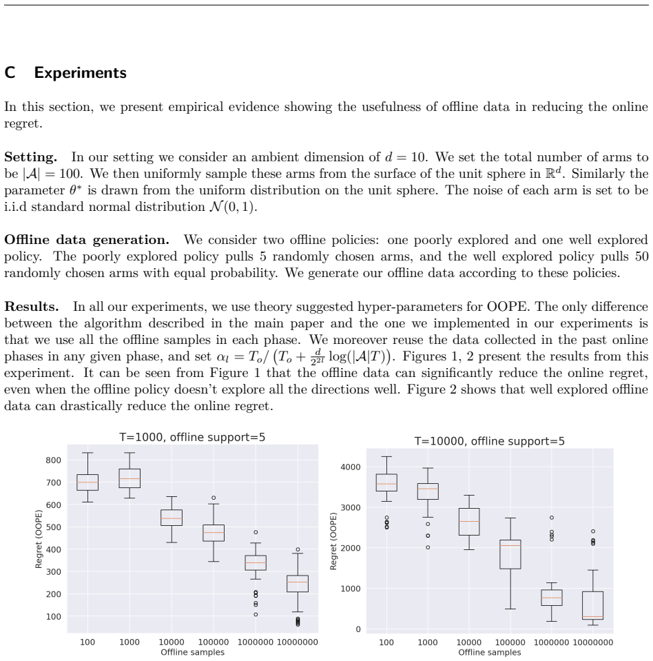
arxiv: 2508.08420 · v3 · submitted 2025-08-11 · 💻 cs.LG · stat.ML

Regret minimization in Linear Bandits with offline data via extended D-optimal exploration

Sushant Vijayan , Arun Suggala , Karthikeyan Shanmugam , Soumyabrata Pal This is my paper

Pith reviewed 2026-05-18 23:15 UTC · model grok-4.3

classification 💻 cs.LG stat.ML

keywords linear banditsregret minimizationoffline dataD-optimal designphased eliminationeffective dimensionbandit exploration

0 comments p. Extension

The pith

An algorithm called OOPE uses extended D-optimal designs in phased elimination to make linear bandit regret scale with the effective dimension of any available offline data.

A machine-rendered reading of the paper's core claim, the machinery that carries it, and where it could break.

The paper shows how to blend existing offline observations into the online exploration process for linear bandits. It defines an effective dimension deff from the eigenvalues of the offline data's Gram matrix to quantify how many directions remain poorly covered. The OOPE algorithm runs exploration phases that solve an extended D-optimal design problem at each step, directing new samples only toward those uncovered directions. This produces a regret bound that shrinks when offline data already covers most of the space and reverts to the usual online bound when the offline data covers nothing new. Matching lower bounds are given for the two extreme regimes of offline quality.

Core claim

Offline-Online Phased Elimination achieves online regret Õ(√(deff T log(|A|T)) + d²) by solving an extended D-optimal design inside each exploration phase; deff is computed directly from the eigen-spectrum of the Gram matrix formed by the offline samples and is at most d. When deff is close to d the bound matches the best known purely online regret; when offline data is abundant and well-spread so that deff is small the additive online cost drops sharply. The same work supplies the first minimax lower bounds that depend explicitly on this offline quality measure and shows that the upper bound is tight in both the well-explored and poorly-explored extremes. A Frank-Wolfe approximation further

What carries the argument

Extended D-optimal design, which augments the classical determinant-maximization criterion with the inverse of the offline Gram matrix so that each new action is chosen to shrink uncertainty only in the directions still poorly covered by prior data.

If this is right

When offline data is abundant and well-spread the online exploration cost can be driven far below the standard √(d T) rate.
The algorithm recovers the classic online regret bound whenever the offline data leaves all directions poorly covered.
A practical Frank-Wolfe solver for the design step reduces the additive d² term to O(d²/deff · min(deff,1)).
The lower bounds prove that no algorithm can do better than OOPE in the two extreme regimes of offline quality.

Where Pith is reading between the lines

These are editorial extensions of the paper, not claims the author makes directly.

Deployments that already hold diverse historical logs could run far fewer live experiments before reaching good performance.
The same coverage measure might be used to decide whether to collect more offline data before switching to online learning.
The phased structure suggests a natural way to interleave new offline batches as they arrive without restarting the entire procedure.

Load-bearing premise

The linear model is exact and the eigenvalues of the offline Gram matrix alone correctly measure coverage quality, without any further conditions on how the offline samples were collected.

What would settle it

A simulation or real deployment in which measured regret stays high even after adding large volumes of offline data whose smallest eigenvalues grow, or in which regret falls below the stated lower bound when deff is shown to be small.

Figures

Figures reproduced from arXiv: 2508.08420 by Arun Suggala, Karthikeyan Shanmugam, Soumyabrata Pal, Sushant Vijayan.

**Figure 1.** Figure 1: (Poorly explored offline policy) Plot showing the utility of offline data when the offline policy is poorly explored (i.e., it doesn’t explore all directions in the action space). The offline data is collected by randomly pulling randomly chosen 5 arms equal number of times. The number of online rounds is T = 103 in the left plot nad T = 104 in the right plot. 51 [PITH_FULL_IMAGE:figures/full_fig_p051_1.png] view at source ↗

**Figure 2.** Figure 2: (Well explored offline policy) Plot showing the utility of offline data when the offline policy is well explored. The offline data is collected by randomly pulling randomly chosen 50 arms equal number of times. The number of online rounds is T = 103 in the left plot nad T = 104 in the right plot. 52 [PITH_FULL_IMAGE:figures/full_fig_p052_2.png] view at source ↗

read the original abstract

We consider the problem of online regret minimization in linear bandits with access to prior observations (offline data) from the underlying bandit model. There are numerous applications where extensive offline data is often available, such as in recommendation systems, online advertising. Consequently, this problem has been studied intensively in recent literature. Our algorithm, Offline-Online Phased Elimination (OOPE), effectively incorporates the offline data to substantially reduce the online regret compared to prior work. To leverage offline information prudently, OOPE uses an extended D-optimal design within each exploration phase. OOPE achieves an online regret is $\tilde{O}(\sqrt{\deff T \log \left(|\mathcal{A}|T\right)}+d^2)$. $\deff \leq d)$ is the effective problem dimension which measures the number of poorly explored directions in offline data and depends on the eigen-spectrum $(\lambda_k)_{k \in [d]}$ of the Gram matrix of the offline data. The eigen-spectrum $(\lambda_k)_{k \in [d]}$ is a quantitative measure of the \emph{quality} of offline data. If the offline data is poorly explored ($\deff \approx d$), we recover the established regret bounds for purely online setting while, when offline data is abundant ($\Toff >> T$) and well-explored ($\deff = o(1) $), the online regret reduces substantially. Additionally, we provide the first known minimax regret lower bounds in this setting that depend explicitly on the quality of the offline data. These lower bounds establish the optimality of our algorithm in regimes where offline data is either well-explored or poorly explored. Finally, by using a Frank-Wolfe approximation to the extended optimal design we further improve the $O(d^{2})$ term to $O\left(\frac{d^{2}}{\deff} \min \{ \deff,1\} \right)$, which can be substantial in high dimensions with moderate quality of offline data $\deff = \Omega(1)$.

Editorial analysis

A structured set of objections, weighed in public.

Desk editor's note, referee report, simulated authors' rebuttal, and a circularity audit. Tearing a paper down is the easy half of reading it; the pith above is the substance, this is the friction.

Desk Editor's Note private letter to a colleague

The paper's real contribution is the first explicit minimax lower bounds for linear bandits that track offline data quality through the Gram matrix spectrum, paired with an algorithm whose regret adapts via an effective dimension deff.

read the letter

The main takeaway is that this work makes the online regret depend on how well the offline data covers the feature space. They define deff from the eigenvalues of the offline Gram matrix to count poorly explored directions, then give an upper bound of Õ(√(deff T log(|A|T)) + d²) for their OOPE algorithm that runs phased elimination with an extended D-optimal design. When offline data is weak, deff is close to d and the bound recovers the usual online linear bandit rate; when offline data is strong, deff shrinks and the online cost drops. They also supply matching lower bounds in the two extreme regimes, which is new for this setting. The Frank-Wolfe approximation to the design further trims the additive d² term to O(d²/deff ⋅ min{deff,1}), which could matter in moderate dimensions. That combination of adaptive upper bound, explicit dependence on offline spectrum, and lower bounds in the extremes is the clearest advance. The analysis appears to derive the bounds directly from the design choice rather than post-hoc fitting, which is a plus. The main soft spot is whether the Frank-Wolfe approximation error is carried all the way through the concentration and elimination steps. Phased elimination proofs usually need the design to satisfy tight optimality conditions on directional variance; an approximate solver with a constant-factor gap can inject an extra additive term if that gap is not controlled. If the paper only shows the improvement at the design level without propagating the error, the claimed reduction may not hold for intermediate deff values. The linear model and standard noise assumptions look fine, but the abstract leaves the precise action-set and noise conditions implicit. This paper is aimed at researchers working on linear bandits and hybrid offline-online learning. A reader who cares about regret bounds that reflect real data coverage will find the deff construction and the lower-bound dependence useful. It is worth sending to a serious referee because the core claims are stated cleanly, the lower bounds are novel, and the algorithmic idea is straightforward even if the approximation detail needs checking.

Referee Report

1 major / 2 minor

Summary. The paper proposes the Offline-Online Phased Elimination (OOPE) algorithm for linear bandits with access to offline data. It incorporates offline observations via an extended D-optimal design computed from the offline Gram matrix, defines an effective dimension deff ≤ d from the eigen-spectrum (λk) of that matrix to quantify poorly covered directions, and claims a regret upper bound Õ(√(deff T log(|A|T)) + d²). The work also states matching minimax lower bounds that depend on offline quality and, via a Frank-Wolfe approximation to the design, improves the additive term to O(d²/deff ⋅ min{deff,1}). Optimality is claimed in the well-explored (deff = o(1)) and poorly-explored (deff ≈ d) regimes.

Significance. If the stated bounds and their optimality hold, the result gives a concrete, data-dependent measure of how offline data reduces online regret in linear bandits, recovering the classic Õ(d√T) bound when offline coverage is absent and yielding substantial savings when offline data is abundant and well-conditioned. The explicit lower bounds that track offline quality are a notable contribution; the Frank-Wolfe improvement, if rigorously justified, would be practically relevant in high-d regimes with moderate deff.

major comments (1)

[Abstract and regret analysis] Abstract and the regret-analysis section: the claimed improvement from O(d²) to O(d²/deff ⋅ min{deff,1}) rests on replacing the exact extended D-optimal design with a Frank-Wolfe approximate solution. Standard phased-elimination analyses require the design to satisfy precise optimality conditions (e.g., uniform bound on the maximum directional variance or on the inverse Gram norm in the poorly covered subspace). The manuscript must explicitly propagate the Frank-Wolfe duality-gap or (1-1/e)-style approximation error through the concentration and elimination arguments; otherwise an extra additive term linear in the design error appears and the stated improvement does not hold for moderate deff = Ω(1).

minor comments (2)

[Notation and definitions] The precise definition of deff in terms of the eigenvalues λk of the offline Gram matrix should be stated as an explicit formula (e.g., deff = ∑_{k=1}^d 1/(1+λk) or the analogous expression used in the analysis) rather than left as a verbal description.
[Model section] Assumptions on the reward noise (sub-Gaussian parameter, etc.) and on the action set A should be stated clearly at the beginning of the model section; the abstract refers to them only implicitly.

Simulated Author's Rebuttal

1 responses · 0 unresolved

We thank the referee for their careful reading of the manuscript and for highlighting this important point in the analysis. We address the comment below and will make the corresponding revisions to strengthen the rigor of the regret bounds.

read point-by-point responses

Referee: [Abstract and regret analysis] Abstract and the regret-analysis section: the claimed improvement from O(d²) to O(d²/deff ⋅ min{deff,1}) rests on replacing the exact extended D-optimal design with a Frank-Wolfe approximate solution. Standard phased-elimination analyses require the design to satisfy precise optimality conditions (e.g., uniform bound on the maximum directional variance or on the inverse Gram norm in the poorly covered subspace). The manuscript must explicitly propagate the Frank-Wolfe duality-gap or (1-1/e)-style approximation error through the concentration and elimination arguments; otherwise an extra additive term linear in the design error appears and the stated improvement does not hold for moderate deff = Ω(1).

Authors: We agree that the current version of the manuscript does not provide a fully explicit propagation of the Frank-Wolfe approximation error through the phased-elimination analysis. In the revised manuscript we will add a dedicated lemma that bounds the deviation between the approximate and exact extended D-optimal designs. Using the standard (1-1/e) guarantee of Frank-Wolfe together with the eigen-structure of the offline Gram matrix, we show that the resulting perturbation in the maximum directional variance (and in the inverse Gram norm restricted to the poorly-covered subspace) contributes an additive term that is absorbed into the improved O(d²/deff ⋅ min{deff,1}) bound. The concentration and elimination arguments are updated accordingly so that no extra linear-in-design-error term appears for deff = Ω(1). We will also clarify the precise optimality conditions that the approximate design continues to satisfy up to a controllable multiplicative factor. revision: yes

Circularity Check

0 steps flagged

No circularity: regret bounds derived directly from algorithm and design properties

full rationale

The paper defines deff explicitly from the eigenvalues of the offline Gram matrix and derives the regret bound for OOPE from the phased elimination procedure combined with the extended D-optimal design properties. The Frank-Wolfe step is presented as a computational approximation to obtain the improved additive term, with the base bound holding independently. No step reduces by construction to a fitted parameter renamed as a prediction, nor does any load-bearing claim rest on a self-citation chain that itself assumes the target result. The derivation remains self-contained against the stated linear model and offline data assumptions.

Axiom & Free-Parameter Ledger

0 free parameters · 2 axioms · 0 invented entities

The central regret claim rests on the linear reward model, bounded noise, and the definition of deff from the offline Gram matrix eigenvalues. No new entities are postulated.

axioms (2)

domain assumption Rewards are linear in action features plus sub-Gaussian noise.
Standard assumption invoked to derive regret bounds for linear bandits.
domain assumption The offline data Gram matrix eigenvalues correctly quantify coverage of feature directions.
Central to the definition of deff and the regret scaling.

pith-pipeline@v0.9.0 · 5916 in / 1299 out tokens · 28541 ms · 2026-05-18T23:15:28.432775+00:00 · methodology

discussion (0)

Reference graph

Works this paper leans on

14 extracted references · 14 canonical work pages

[1]

αl max a∈S πoff(a)< αlπoff(S)+(1−αl) |S|

work page
[2]

αlπoff(S)+(1−αl) |S| ≤(1−αl) +αlmin a∈S πoff(a)

work page
[3]

We shall now restrict our search ofS to sets of the following form: Si ={a∈Al |πoff(a)≤πoff(i)} for somei∈[r]

αlπoff(S)+(1−αl) |S| ≤αl min a∈Al\S πoff(a) then S is the support set ofπ∗ l,on and for alla∈S we have that: π∗ l,on(a) = 1 |S|+ αl 1−αl [πoff(S) |S|−πoff(a) ] and g(˜π⋆ l ) = |S| αlπoff(S) + (1−αl). We shall now restrict our search ofS to sets of the following form: Si ={a∈Al |πoff(a)≤πoff(i)} for somei∈[r]. Writing out the three properties to be satisfi...

work page
[4]

In case for somek,i∈[d] if ck,i = 0 then we haveA+ ck,i =A− ck,i

work page
[5]

If ck,i̸= 0, then we have that the setsA+ ck,i,A− ck,i are disjoint. 32 Now let us define ad(d−1)/2 collection Aij of d×d matrices indexed by the ordered pair(i,j ),i,j ∈[d] with i<j as follows: Aij k,l =πoff(A+ ck,i∩A+ cl,j) +πoff(A− ck,i∩A− cl,j)−πoff(A+ ck,i∩A− cl,j)−πoff(A− ck,i∩A+ cl,j). for k,l∈[d]. Now we state a useful lemma: Lemma A.4.Given that|...

work page
[6]

(Coordinate Independence).∀i,j,k,l ∈[d] πoff(Ai =ck,i,Aj =cl,j) =πoff(Ai =ck,i)πoff(Aj =cl,j)

work page
[7]

33 Proof

(±Symmetricity).∀i,k∈[d] πoff(Ai =ck,i) =πoff(Ai =−ck,i) , that is,πoff is independent co-ordinate wise and symmetrically distributed wrt to positive & negative values of a componentck,i, then we have thatAij = 0 for alli<j . 33 Proof. From coordinate independence we have that: πoff(A+ ck,i∩A+ cl,j) =πoff(A+ ck,i)πoff(A+ cl,j) πoff(A− ck,i∩A− cl,j) =πoff(...

work page
[8]

The optimization definingdlb e in equation (37) is a concave program inw

work page
[9]

If ∑d i=1vi = 1, v1 =v2 =···=vk−1 = 0 and 0<v k≤vk+1≤···≤vd, for somek∈[d] then: dlb e = (k−1) + (d−k + 1)√ 1 + Toff T 36 We provide a dual representation ofdlb e in the next lemma: Lemma A.9 (Dual representation ofdlb e ). For simplicity assume that0 < v1≤···≤vd.Define for each i∈[d], the following functions: βi(x) =    vi, for x≤ −Toff 2Tvi(1+ ...

work page 1997
[10]

The optimal solutionH∗ α(V,d ) to the primal problemP(V,α,d) is feasible for the primal problem P ( V, 0, d−αTr(H∗ α(V,d)Vπoff) 1−α )

work page
[11]

The optimal solutionH∗ 0 (V,d ) to the primal problemP(V, 0,d ) is feasible for the primal problem P(V,α,d). Proof. (1) As H∗ α(V,d ) is feasible forP(V,α,d) we have that (1−α)atH∗ α(V,d )a +αTr(H∗ α(V,d )Vπoff)≤d for alla∈V. Thus by simple manipulation of terms we have atH∗ α(V,d )a≤d−αTr(H∗ α(V,d )Vπoff) 1−α . We observe thatd > αTr(H∗ α(V,d )Vπoff) and...

work page 2016
[12]

m(δ) is increasing ifδ≥0 and decreasing ifδ <0

work page
[13]

for δ≥δ0, m(δ)≥ ( 1− δ0 (1+δ0)(ln(1+δ0) ) ln(1 +δ)

work page
[14]

B.5 Proof of Proposition 5.5

for|δ|≤1/2, m(δ)≥2/7δ2. B.5 Proof of Proposition 5.5. Proof. Consider an iterateπ(t) l such thatδ(π(t) l )≥1. Setγt =d(π∗ l,on,Al,α)−d(π(t) l ,Al,α). Then γt−γt+1 =d(π(t+1) l ,Al,α)−d(π(t) l ,Al,α) ≥log(1 +δ(π(t) l ))−δ(π(t) l ) 1 +δ(π(t) l ) ≥ ( 1− δ0 (1 +δ0)(ln(1 +δ0) ) log(1 +δ(π(t) l )) ≥ (1 d− δ0 d(1 +δ0)(ln(1 +δ0) ) γ. 49 The first inequality follow...

work page