REVIEW 4 major objections 5 minor 2 cited by
An all-sky 3D dust map Based on Gaia and LAMOST
T0 review · 4 major / 5 minor · reviewed 2026-08-04 · deepseek-v4-flash
Pith's one-line read By merging ~0.01-mag spectroscopic reddening from LAMOST with ~150 million Gaia XP-based measurements, the authors build an all-sky 3D map whose per-sightline fit separates the local bubble, the diffuse dust layer, and up to four molecular
desk verdict A useful all-sky 3D reddening map that will get adopted, but the headline 0.01 mag precision is fit residual, not validated absolute accuracy. read the letter →
The pith
A machine-rendered reading of the paper's core claim, the machinery that carries it, and where it could break.
The reading
What carries the argument
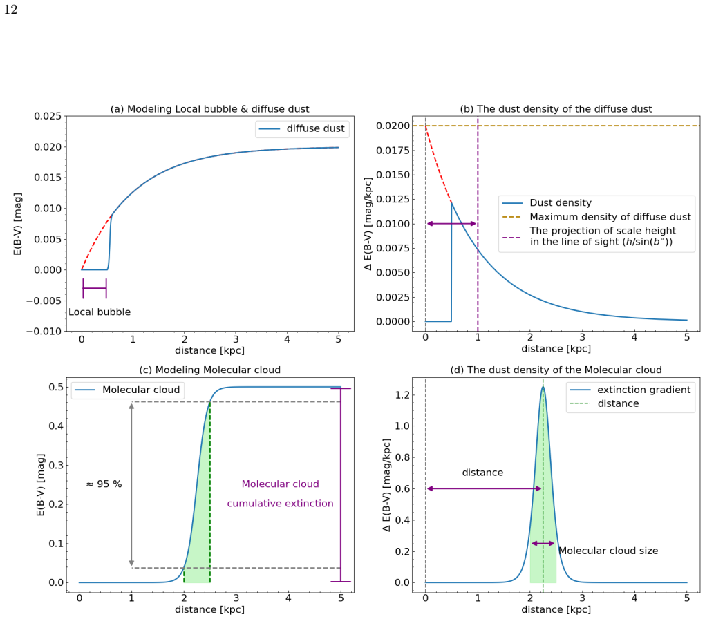
The carrying mechanism is the parametric line-of-sight model of Section 3.2 (Eqs. 2-4, 8-9): total E(B-V) equals a diffuse interstellar medium term - zero inside a fitted local-bubble boundary, then exponential decay with fitted scale height and density - plus up to four 'modified sigmoid' clouds, each with a distance d_MC, a line-of-sight width Lambda_MC, and cumulative reddening Delta E(B-V)_MC. The sigmoid is the workhorse: smooth, with an analytic derivative, so one fit yields both the reddening curve and the dust-density profile in mag/kpc, with cloud peaks readable directly. An L1 penalty (lambda=0.1) on cloud amplitudes drives superfluous clouds to zero, making model selection part of
What would settle it
Compare lines of sight through well-studied complexes (e.g., the Aquila Rift and the Perseus region) against 3D dust inversions built without this parametric prior, and against maser-parallax or CO-based cloud distances. If the fitted cloud distances disagree with independent distances beyond combined uncertainties, or if the inversion shows peaks or wings the four-sigmoid form cannot absorb, the map's structure is an artifact of the assumed shape. A second check follows from the paper's own concession that cloud widths are distance-dominated: fitting only stars with the most precise parallaxe
Extended reading notes
Core claim
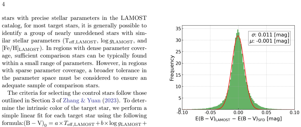
One data product can give, for any direction, a continuous reddening-distance curve whose parts are separately identifiable: a dust-free local bubble, an exponential diffuse dust layer, and up to four molecular clouds, each with fitted distance, width, and reddening. Two independent estimators - LAMOST standard-pair reddening (~0.01 mag) and Gaia XP forward-model reddening - are cross-validated; XP is aligned by 0.89; ~150 million sources are kept; and an L1-regularized weighted absolute-deviation fit makes redundant clouds vanish. The resulting all-sky map runs at 3.4-58 arcmin resolution (half the sky better than 6.9 arcmin), reaches 10-15 kpc off-plane and 3-5 kpc in-plane, with ~0.01 mag
Load-bearing premise
The load-bearing premise is that every line of sight is exactly a dust-free local bubble, an exponentially thinning diffuse layer, and at most four smooth, symmetric cloud steps. Wherever real dust deviates from this shape, the fitted cloud distances, cloud widths, and scale height are biased even if total reddening is right; the paper itself concedes cloud widths are dominated by distance errors, and that the XP non-negativity offset can bias the high-latitude scale height.
Editorial extensions
If this is right
- Any star behind the map can be corrected for foreground reddening with typical 0.01-0.03 mag precision and arcminute-scale resolution, including low-latitude directions where previous all-sky maps are coarser.
- The fitted components themselves become data: the local-bubble boundary, the diffuse-dust scale height, and the distance, width, and cumulative reddening of up to four molecular clouds are returned for every direction, enabling cloud-distance and dust-structure studies without re-deriving the map.
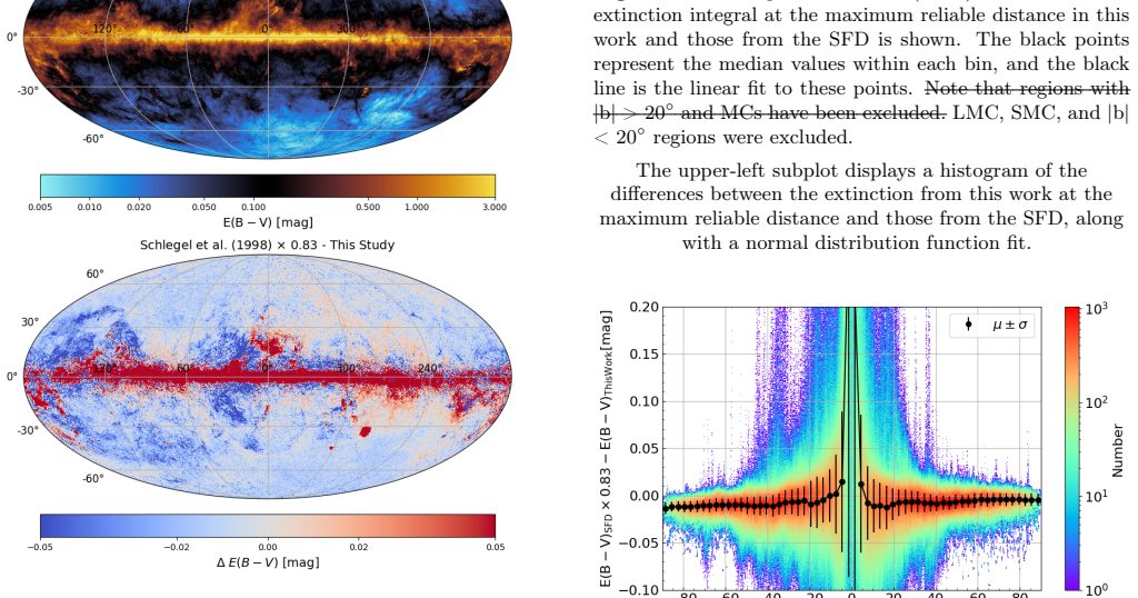
- Integrated to its maximum reliable distance, the map confirms SFD's reddening is about 16% too high (scale factor 0.834) and agrees with SFD at high Galactic latitude while adding finer detail; it also finds reddening in high-latitude regions where the Green et al. (2019) map reads zero.
- The comparison with Green et al. (2019) reveals previously unnoticed structures - prominent molecular clouds at 0.5-1 kpc at high latitude and features extending out of the disk at 0.5-2 kpc - which the authors flag for follow-up.
- The public website and Python package (pip install dustmaps3d) let a user query extinction, dust density, uncertainty, maximum reliable distance, local-bubble distance, diffuse scale height, and cloud membership for any three-dimensional position.
Reading between the lines
- My reading: the per-sightline cloud components amount to an implicit all-sky catalog of molecular-cloud distances; the natural check the paper does not perform is comparing fitted d_MC against independent distances (maser parallaxes or CO kinematics) for well-known complexes such as Orion, Perseus, and the Aquila Rift.
- My reading: the absolute zero-point of the whole map hangs on the standard-pair assumption that stars sharing atmospheric parameters share intrinsic color; users doing precision work should treat the 0.89 (XP-to-LAMOST) and 0.834 (LAMOST-to-SFD) scale factors as a chain that could carry a small systematic tilt across stellar types.
- My reading: a discriminating null test of the parametric form is to run a non-parametric tomographic inversion on the lines of sight with the worst residuals (low latitude, high cloud count); if an inversion reveals structure the four-sigmoid form cannot express, the cloud-count ceiling and sigmoid shape, not the data, set the map's structural limit.
- My reading: the in-plane distance limit (3-5 kpc) is set by the faint end of the XP sample rather than by the method, so the same pipeline could be re-run on deeper surveys to push deeper into the dust disk, and the parametric design makes such updates cheap.
Signed reviews
Editorial analysis
A structured set of objections, weighed in public.
Referee Report
Summary. The paper constructs an all-sky 3D dust reddening map by combining LAMOST DR11 standard-pair E(B−V) measurements (~4.6 million stars) with Gaia XP–based extinctions from Zhang et al. (2023a), rescaled and filtered to ~150 million sources with revised Gaia distances. An adaptive HEALPix partition yields sightlines of 3.4′–58′ resolution, and each sightline is fit with a parametric distance–reddening model consisting of a dust-free local bubble, an exponential diffuse ISM, and up to four modified-sigmoid molecular clouds under an L1 penalty. The abstract claims typical individual-star reddening precision of ~0.01 mag at |b|>20° and 0.01–0.05 mag at lower latitudes, with distance coverage of 3–5 kpc in the plane and 10–15 kpc elsewhere. The paper also provides public data products and comparisons to SFD and Green et al. (2019).
Significance. If the precision and coverage claims hold, this would be a valuable community resource: the largest all-sky 3D reddening map with arcminute-class resolution, built from ~150 million stars, with per-sightline parameters for the local bubble, diffuse dust, and molecular clouds. The paper's strengths include careful cross-matching and filtering of LAMOST and Gaia XP data, public release of the map and Python tools, and external anchors that are broadly reassuring: the SFD scaling factor of 0.834 (§4.2.1) is consistent with earlier independent calibrations, and the large-scale comparisons with Green et al. (2019) show good agreement. However, the headline precision is currently an in-sample, post-clipping fit residual, and the DIM model contains a sign error for southern Galactic latitudes. These issues are load-bearing for the central claims, so the paper needs a substantial revision before the quantitative results can be accepted.
major comments (4)
- [§3.2, Eqs. (3) and (8)] The DIM term is written with h/sin b and no absolute value. For any sightline with b<0, h/sin b<0, so 1−exp(−d/(h/sin b)) grows without bound as d increases, and the derivative in Eq. (8) becomes an increasing exponential. This is unphysical and affects every southern Galactic latitude sightline; b=0 is also singular. Replace sin b by |sin b| (or sin|b|) in Eqs. (3) and (8), refit all affected lines of sight, and recompute the southern-sky results in Figs. 15–20 and the public data products. This is load-bearing because the map is advertised as all-sky.
- [§3.3 and §4.1] The quoted ~0.01 mag reddening precision is the standard deviation of residuals of the model fitted to the same stars that define each line of sight, after iterative 3σ clipping. With up to 15 free parameters per sightline (Eqs. 3–9) and λ=0.1 in Eq. (15), in-sample residuals measure internal consistency, not predictive error. Please add a hold-out validation, e.g., fit each sightline on a random half of the stars and report σ on the held-out half, binned by |b|, distance, and cumulative E(B−V), or compare per-star predictions against an independent reddening catalog at matched distances. Without this, the headline precision is not established.
- [§2.3] The rescaled XP extinctions (factor 0.89) and the adopted XP errors are calibrated against the same LAMOST standard-pair reference that is itself part of the final dataset, and Z23's XP model used LAMOST parameters for training. This is partially an intra-family validation. Although the final SFD factor 0.834 agrees with earlier independent calibrations, the per-star error model is not independently tested. Please validate the rescaled XP E(B−V) against an independent spectroscopic or photometric reference (e.g., APOGEE/RAVE or red-clump colors), and quantify how the non-negativity offset described at the end of §2.3 propagates into the high-latitude DIM scale height.
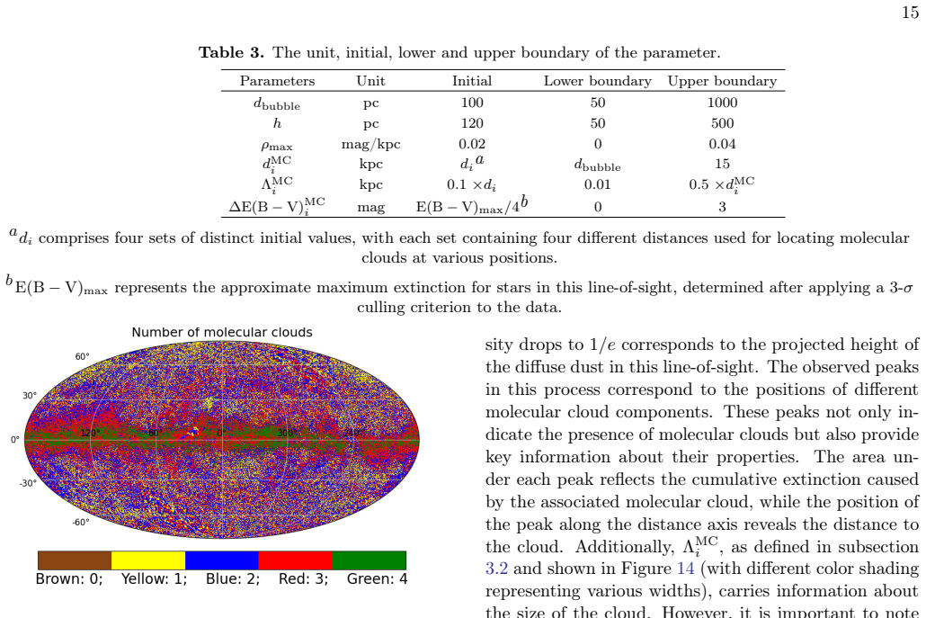
- [§3.2, §4.1, §5] The public tool exposes cloud distances, cloud widths Λ_MC_i, and DIM scale height h as physical parameters, but §4.1 concedes that cloud widths are dominated by distance uncertainties, and §2.3 concedes that the Z23 offset can bias h. This undermines the parametric interpretability claim unless (i) Λ_MC_i is reported as an apparent width with a deconvolved estimate or clear caveat, and (ii) cloud distances are validated against known nearby clouds (e.g., Orion, Taurus, Perseus, California) or existing dust maps. The sensitivity to the ad hoc λ=0.1 in Eq. (15) should also be tested, since the number of retained clouds depends on it.
minor comments (5)
- [§3.1, after Eq. (1)] The sentence 'and a and b αandβ are parameters' is garbled; it should read 'α and β are parameters.'
- [§2.2] In the definition of E(B−V)_LAMOST, the text says 'E(B−V)_observed is the observed color'; this should be '(B−V)_observed'.
- [§6 and elsewhere] Several occurrences of 'Milk Way' should be 'Milky Way'.
- [Figure 15] The lower panels compare the authors' residual σ with σ values 'calculated from the extinction curves provided by Green et al. (2019).' Please describe how those σ values are computed (same distance bins, same stars, or map-to-map scatter) so the comparison is interpretable.
- [§4.1] The 'maximum reliable distance' is defined as the distance to the farthest star in each sightline after 3σ clipping. This is not an independent completeness or sensitivity limit; please state this caveat explicitly or provide a recovery test.
Circularity Check
No circular derivation: the map is an independent fit with external support; the headline precision is an in-sample residual (validation caveat) and the SFD comparison partly inherits the input 0.86 scaling, but these are not circular reductions.
full rationale
The central derivation is self-contained: E(B−V)_LAMOST is obtained by standard-pair interpolation on low-SFD control stars; E(B−V)_XP comes from the Zhang et al. (2023a) forward model; the two are cross-calibrated with a fitted 0.89 factor (§2.3) and then a parametric local-bubble + exponential-DIM + up-to-4-cloud model is fit per sightline (§3). This is a genuine fit, not an identity. External comparisons with Green et al. (2019) and SFD (§4.2) provide independent large-scale support. The main caveats are validation issues, not circularity: the quoted 0.01–0.05 mag precision is the residual σ of the fit to the same stars, after iterative 3σ clipping (§3.3, §4.1), so it is an in-sample estimate; hold-out validation would be needed to confirm predictive error. The SFD comparison in §4.2.1 partly inherits the 0.86 SFD scaling used to define intrinsic colors in §2.2, so the 0.834 ratio is not fully independent, but the paper cites prior calibrations and does not use 0.834 to construct the map. Self-citations (e.g., Yuan et al. 2013; Zhang & Yuan 2023; Sun et al. 2022) are methodological and not load-bearing; no uniqueness-theorem or ansatz-by-citation pattern is present. The paper also explicitly concedes that cloud widths are dominated by distance uncertainties (§4.1) and that Z23's non-negativity offset can bias high-latitude scale heights (§2.3); these are acknowledged limitations, not circular steps.
Assumptions & free parameters
free parameters (8)
- XP scale factor =
0.89
- L1 regularization lambda =
0.1
- Decentration weight parameters alpha, beta =
alpha=7.5, beta=-5
- Per-sightline DIM parameters d_bubble, h, rho_max =
bounds: 50-1000 pc, 50-500 pc, 0-0.04 mag/kpc
- Per-cloud parameters d_MC, Lambda_MC, DeltaE_MC =
up to 4 clouds per sightline, 4 multi-start initial sets
- Z23 reliability cuts =
quality flag<8, teff_confidence>0.2, SNR_BP>5, SNR_RP>7
- Weight caps and normalization =
E(B-V)_err 0.01-0.1 mag; relative distance error 0.5%-50%
- 3-sigma clipping threshold =
3-sigma, iterative, with re-fit
assumptions (7)
- domain assumption Stars with identical (Teff, log g, [Fe/H]) have identical intrinsic (B-V)
- domain assumption Control stars with E(B-V)_SFD < 0.01 mag are unreddened after a 0.86 rescale of SFD
- domain assumption DIM density falls exponentially with Galactic height and the Local Bubble is dust-free
- domain assumption Molecular clouds are modified sigmoid profiles with central maximum density
- ad hoc to paper At most 4 significant clouds per sightline (n=4) with lambda L1 penalty
- domain assumption LAMOST stellar parameters are extinction-independent because they are derived from normalized spectra
- domain assumption Z23 revised parallaxes (inverse-parallax distances) and Bailer-Jones geometric distances are unbiased and interchangeable
Cite this review
Pith. "Pith review of An all-sky 3D dust map Based on Gaia and LAMOST." pith.science (2026). https://pith.science/paper/763PLKS5
@misc{pith2026250907640,
  author       = {Pith},
  title        = {Pith review of: An all-sky 3D dust map Based on Gaia and LAMOST},
  year         = {2026},
  howpublished = {\url{https://pith.science/paper/763PLKS5}},
  note         = {Machine review of arXiv:2509.07640}
}
abstract
We present a comprehensive 3D dust reddening map covering the entire Milky Way, constructed by combining reddening estimates based on LAMOST low-resolution spectra (E(B$-$V)$_{\rm LAMOST}$) with those derived from $Gaia$ XP spectra (E(B$-$V)$_{\rm XP}$), along with revised $Gaia$ distances. E(B$-$V)$_{\rm LAMOST}$ values of $\sim$ 4.6 million unique sources were obtained with the standard-pair analysis using LAMOST DR11 stellar parameters and synthesized $B/V$-band photometry from $Gaia$ XP spectra, showing a typical precision of $\sim$ 0.01 mag. The E(B$-$V)$_{\rm XP}$ from the catalog of \citet{zhang2023}, which was derived using forward modeling of $Gaia$ XP spectra, were cross-validated with E(B$-$V)$_{\rm LAMOST}$, leading to the selection of $\sim$ 150 million high-reliability measurements. The combined dataset achieves a median precision of $\sim$ 0.03 mag for E(B$-$V). To model the reddening -- distance relationship along various lines-of-sight, we implemented a parametric approach that accounts for contributions from the local bubble, diffuse interstellar-medium, and multiple potential molecular clouds. The sky was adaptively partitioned based on stellar density, resulting in angular resolutions ranging from 3.4$^{\prime}$ to 58$^{\prime}$, with about half of the sky having a resolution better than 6.9$^{\prime}$. The reddening precision of our 3D map for individual stars reaches $\sim$ 0.01 mag in most regions at $|b| > 20^\circ$, but degrades to 0.01-0.05 mag at $|b| < 20^\circ$. The map reaches a maximum distance of 3-5 kpc in high-extinction regions with $|b| < 5^\circ$, and extends to 10-15 kpc elsewhere. An interactive platform and Python package have been developed for utilization of the 3D dust map. Available online: https://nadc.china-vo.org/data/dustmaps/.
Figures


Figures from the paper (15 more)






Forward citations
Cited by 2 Pith papers
-
Milky Way Atlas: A radial-velocity-resolved, three-dimensional map of H I within 1.25 kpc
A Bayesian inference method combining HI4PI radio data with Gaia-based 3D dust maps reconstructs the 3D density, velocity, and line-width of local atomic hydrogen within 1.25 kpc, validated by synthetic tests and inde...
-
Unveiling the nature of G6096: a likely hierarchical triple system
G6096 is likely a hierarchical triple of main-sequence stars rather than a binary hosting a white dwarf or neutron star.
Reference graph
Works this paper leans on
-
[1]
An, D., Beers, T. C., & Chiti, A. 2024, ApJS, 272, 20, doi: 10.3847/1538-4365/ad3641
-
[2]
2021, AJ, 161, 147, doi: 10.3847/1538-3881/abd806
Demleitner, M., & Andrae, R. 2021, AJ, 161, 147, doi: 10.3847/1538-3881/abd806
-
[3]
Chen, B. Q., Schultheis, M., Jiang, B. W., et al. 2013, A&A, 550, A42, doi: 10.1051/0004-6361/201219682
-
[4]
Chen, B. Q., Huang, Y., Yuan, H. B., et al. 2019, MNRAS, 483, 4277, doi: 10.1093/mnras/sty3341
-
[5]
Cox, D. P., & Reynolds, R. J. 1987, ARA&A, 25, 303, doi: 10.1146/annurev.aa.25.090187.001511
arXiv 1987
-
[6]
Cui, X.-Q., Zhao, Y.-H., Chu, Y.-Q., et al. 2012, Research in Astronomy and Astrophysics, 12, 1197, doi: 10.1088/1674-4527/12/9/003 De Angeli, F., Weiler, M., Montegriffo, P., et al. 2023, A&A, 674, A2, doi: 10.1051/0004-6361/202243680
-
[7]
Dharmawardena, T. E., Bailer-Jones, C. A. L., Fouesneau, M., et al. 2024, MNRAS, 532, 3480, doi: 10.1093/mnras/stae1474
-
[8]
Draine, B. T. 2003, ARA&A, 41, 241, doi: 10.1146/annurev.astro.41.011802.094840
arXiv 2003
Show all 39 references
-
[9]
2003, A&A, 409, 205, doi: 10.1051/0004-6361:20031070
Drimmel, R., Cabrera-Lavers, A., & López-Corredoira, M. 2003, A&A, 409, 205, doi: 10.1051/0004-6361:20031070
2003 doi
-
[10]
Drimmel, R., & Spergel, D. N. 2001, ApJ, 556, 181, doi: 10.1086/321556 Ferrière, K. M. 2001, Reviews of Modern Physics, 73, 1031, doi: 10.1103/RevModPhys.73.1031
2001 doi
-
[11]
A., Dettbarn, C., & Flynn, C
Fuchs, B., Breitschwerdt, D., de Avillez, M. A., Dettbarn, C., & Flynn, C. 2006, MNRAS, 373, 993, doi: 10.1111/j.1365-2966.2006.11044.x Gaia Collaboration, Prusti, T., de Bruijne, J. H. J., et al. 2016, A&A, 595, A1, doi: 10.1051/0004-6361/201629272 Gaia Collaboration, Montegr...
2006
-
[12]
2019, ApJ, 887, 93, doi: 10.3847/1538-4357/ab5362
Finkbeiner, D. 2019, ApJ, 887, 93, doi: 10.3847/1538-4357/ab5362
2019 doi
-
[13]
L., Chen, B
Guo, H. L., Chen, B. Q., Yuan, H. B., et al. 2021, ApJ, 906, 47, doi: 10.3847/1538-4357/abc68a
2021 doi
- [14]
-
[15]
Koo, B.-C., & McKee, C. F. 1992, ApJ, 388, 93, doi: 10.1086/171132
1992 doi
-
[16]
L., Babusiaux, C., & Cox, N
Lallement, R., Vergely, J. L., Babusiaux, C., & Cox, N. L. J. 2022, A&A, 661, A147, doi: 10.1051/0004-6361/202142846
2022 doi
-
[17]
L., & Redfield, S
Linsky, J. L., & Redfield, S. 2021, ApJ, 920, 75, doi: 10.3847/1538-4357/ac1feb
2021 doi
-
[18]
W., Yuan, H
Liu, X. W., Yuan, H. B., Huo, Z. Y., et al. 2014, in IAU
2014
-
[19]
298, Setting the scene for Gaia and LAMOST, ed
Symposium, Vol. 298, Setting the scene for Gaia and LAMOST, ed. S. Feltzing, G. Zhao, N. A. Walton, & P. Whitelock, 310–321, doi: 10.1017/S1743921313006510
-
[20]
L., Zhao, Y.-H., Zhao, G., et al
Luo, A. L., Zhao, Y.-H., Zhao, G., et al. 2015, Research in Astronomy and Astrophysics, 15, 1095, doi: 10.1088/1674-4527/15/8/002
2015 doi
-
[21]
2006, A&A, 453, 635, doi: 10.1051/0004-6361:20053842
Picaud, S. 2006, A&A, 453, 635, doi: 10.1051/0004-6361:20053842
2006 doi
-
[22]
McKee, C. F. 1995, in Astronomical Society of the Pacific Conference Series, Vol. 80, The Physics of the Interstellar Medium and Intergalactic Medium, ed. A. Ferrara, C. F
1995
-
[23]
2021, ApJ, 909, 48, doi: 10.3847/1538-4357/abdbac Planck Collaboration, Abergel, A., Ade, P
Niu, Z., Yuan, H., & Liu, J. 2021, ApJ, 909, 48, doi: 10.3847/1538-4357/abdbac Planck Collaboration, Abergel, A., Ade, P. A. R., et al. 2014, A&A, 571, A11, doi: 10.1051/0004-6361/201323195
2021 doi
-
[24]
J., Menten, K
Reid, M. J., Menten, K. M., Brunthaler, A., et al. 2019, ApJ, 885, 131, doi: 10.3847/1538-4357/ab4a11
2019 doi
-
[25]
F., & Finkbeiner, D
Schlafly, E. F., & Finkbeiner, D. P. 2011, ApJ, 737, 103, doi: 10.1088/0004-637X/737/2/103
2011 doi
-
[26]
F., Finkbeiner, D
Schlafly, E. F., Finkbeiner, D. P., Schlegel, D. J., et al. 2010, ApJ, 725, 1175, doi: 10.1088/0004-637X/725/1/1175
2010 doi
-
[27]
J., Finkbeiner, D
Schlegel, D. J., Finkbeiner, D. P., & Davis, M. 1998, ApJ, 500, 525, doi: 10.1086/305772
1998 doi
-
[28]
2022, ApJS, 260, 17, doi: 10.3847/1538-4365/ac642f
Sun, Y., Yuan, H., & Chen, B. 2022, ApJS, 260, 17, doi: 10.3847/1538-4365/ac642f
2022 doi
-
[29]
L., Lallement, R., & Cox, N
Vergely, J. L., Lallement, R., & Cox, N. L. J. 2022, A&A, 664, A174, doi: 10.1051/0004-6361/202243319
2022 doi
-
[30]
2020, A&A, 639, A72, doi: 10.1051/0004-6361/201936868
Wang, S., Zhang, C., Jiang, B., et al. 2020, A&A, 639, A72, doi: 10.1051/0004-6361/201936868
2020 doi
-
[31]
2025, Submitted
Wang, T., Yuan, H., Chen, B., et al. 2025, Submitted
2025
-
[32]
Y., & Shelton, R
Welsh, B. Y., & Shelton, R. L. 2009, Ap&SS, 323, 1, doi: 10.1007/s10509-009-0053-3
2009 doi
-
[33]
L., Li, H.-N., et al
Wu, Y., Luo, A. L., Li, H.-N., et al. 2011, Research in Astronomy and Astrophysics, 11, 924, doi: 10.1088/1674-4527/11/8/006
2011 doi
-
[34]
B., Liu, X
Yuan, H. B., Liu, X. W., & Xiang, M. S. 2013, MNRAS, 430, 2188, doi: 10.1093/mnras/stt039
2013 doi
-
[35]
2023, ApJS, 264, 14, doi: 10.3847/1538-4365/ac9dfa 25
Zhang, R., & Yuan, H. 2023, ApJS, 264, 14, doi: 10.3847/1538-4365/ac9dfa 25
2023 doi
-
[36]
2024, ApJ, 971, 127, doi: 10.3847/1538-4357/ad613e
Zhang, R., Yuan, H., Huang, B., et al. 2024, ApJ, 971, 127, doi: 10.3847/1538-4357/ad613e
2024 doi
-
[37]
M., & Rix, H.-W
Zhang, X., Green, G. M., & Rix, H.-W. 2023a, MNRAS, 524, 1855, doi: 10.1093/mnras/stad1941 —. 2023b, Parameters of 220 million stars from Gaia BP/RP spectra, v1.2, Zenodo, doi: 10.5281/zenodo.7811871
-
[38]
2012, Research in Astronomy and Astrophysics, 12, 723, doi: 10.1088/1674-4527/12/7/002
Zhao, G., Zhao, Y.-H., Chu, Y.-Q., Jing, Y.-P., & Deng, L.-C. 2012, Research in Astronomy and Astrophysics, 12, 723, doi: 10.1088/1674-4527/12/7/002
2012 doi
-
[39]
A., Alves, J., et al
Zucker, C., Goodman, A. A., Alves, J., et al. 2022, Nature, 601, 334, doi: 10.1038/s41586-021-04286-5
2022 doi
Reviewed August 4, 2026 · model on record in the stance chip above.
Discussion (0). Continue with ORCID to comment.