Infusing Experimental Reality into Complex Many-Body Hamiltonians: The Observable-Constrained Variational Framework (OCVF)

Shaoliang Guo; Ziping Yang

arxiv: 2512.10315 · v2 · submitted 2025-12-11 · ❄️ cond-mat.mtrl-sci

Infusing Experimental Reality into Complex Many-Body Hamiltonians: The Observable-Constrained Variational Framework (OCVF)

Shaoliang Guo , Ziping Yang This is my paper

Pith reviewed 2026-05-16 23:52 UTC · model grok-4.3

classification ❄️ cond-mat.mtrl-sci

keywords observable-constrained variational frameworkneural network potentialsBaTiO3phase transitionsmany-body Hamiltoniansexperimental constraintsdeep learning potentialspair distribution function

0 comments

The pith

A variational framework corrects theoretical Hamiltonians with neural terms to match experimental observables and predict accurate phase transitions in BaTiO3.

A machine-rendered reading of the paper's core claim, the machinery that carries it, and where it could break.

The paper introduces the Observable-Constrained Variational Framework to correct a theoretical Hamiltonian H_o by training a neural network term ΔH_θ that enforces agreement with experimental observables such as pair distribution functions. When applied to BaTiO3, the resulting model H_o + ΔH_θ reproduces the complete sequence of phase transitions. It improves the cubic-tetragonal transition temperature accuracy by 95.8 percent, the orthorhombic-rhombohedral by 36.1 percent, and rhombohedral lattice accuracy by 55.6 percent. Readers would care because this provides a practical route to add physical realism to deep learning potentials without discarding the original theory.

Core claim

The central claim is that the Observable-Constrained Variational Framework extends the Constrained-Ensemble Variational Method by training a neural network correction ΔH_θ so the combined Hamiltonian matches experimental observables across temperatures, allowing accurate prediction of BaTiO3's full phase transition sequence with the reported accuracy improvements.

What carries the argument

The Observable-Constrained Variational Framework (OCVF) is a top-down correction method that uses a neural network to learn the functional correction ΔH_θ enforcing match to experimental observables like pair-distribution functions.

If this is right

The augmented Hamiltonian predicts the full temperature-driven phase transition sequence in BaTiO3 accurately.
Cubic-tetragonal transition temperature accuracy rises by 95.8 percent relative to the uncorrected model.
Orthorhombic-rhombohedral transition temperature accuracy rises by 36.1 percent.
Lattice-structure accuracy in the rhombohedral phase rises by 55.6 percent.

Where Pith is reading between the lines

These are editorial extensions of the paper, not claims the author makes directly.

The same constrained-correction approach could be tested on other perovskites where both DFT and experimental PDF data exist.
If the neural correction remains stable under modest changes in training temperature windows, it may indicate that missing physics is being captured rather than memorized.
One could check whether the learned correction functional transfers to different observables such as dielectric constants or elastic moduli.

Load-bearing premise

The neural network correction ΔH_θ trained on experimental PDF data generalizes to new phases and temperatures without overfitting or unphysical artifacts.

What would settle it

Applying the corrected model to independent experimental data for BaTiO3 phase transitions and finding no improvement in accuracy would falsify the claim.

Figures

Figures reproduced from arXiv: 2512.10315 by Shaoliang Guo, Ziping Yang.

**Figure 2.** Figure 2: FIG. 2. Improved DimeNet++ architecture diagram [PITH_FULL_IMAGE:figures/full_fig_p006_2.png] view at source ↗

**Figure 3.** Figure 3: FIG. 3 [PITH_FULL_IMAGE:figures/full_fig_p007_3.png] view at source ↗

**Figure 4.** Figure 4: FIG. 4. Three dimension of correction under 300K [PITH_FULL_IMAGE:figures/full_fig_p008_4.png] view at source ↗

**Figure 5.** Figure 5: FIG. 5. correction to BTO violin plots—derived Phase Transition [PITH_FULL_IMAGE:figures/full_fig_p009_5.png] view at source ↗

**Figure 6.** Figure 6: FIG. 6. the ratio of c-axis of BTO [PITH_FULL_IMAGE:figures/full_fig_p010_6.png] view at source ↗

**Figure 8.** Figure 8: FIG. 8. BTO Polarization Transition [PITH_FULL_IMAGE:figures/full_fig_p010_8.png] view at source ↗

**Figure 9.** Figure 9: FIG. 9 [PITH_FULL_IMAGE:figures/full_fig_p012_9.png] view at source ↗

**Figure 10.** Figure 10: FIG. 10 [PITH_FULL_IMAGE:figures/full_fig_p013_10.png] view at source ↗

read the original abstract

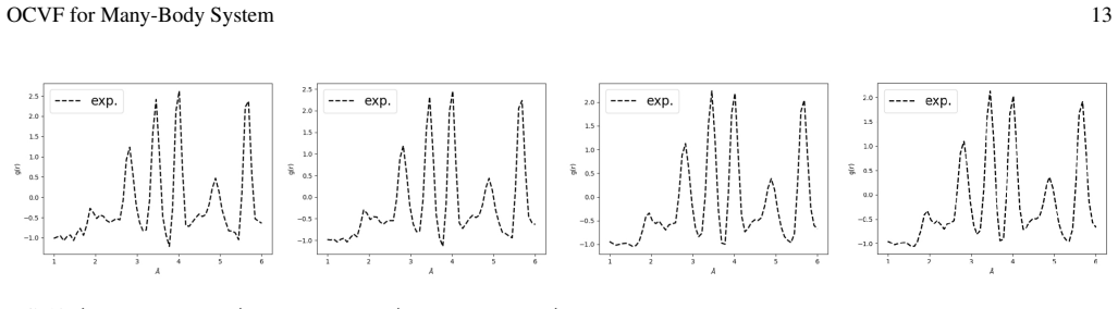
Deep learning potentials for complex many-body systems often face challenges of insufficient accuracy and a lack of physical realism. This paper proposes an "Observable-Constrained Variational Framework" (OCVF), a general top-down correction paradigm designed to infuse physical realism into theoretical "skeleton" models (H_o) by imposing constraints from macroscopic experimental observables (\mathfrak{O}_{\text{exp},s}). We theoretically derive OCVF as a numerically tractable extension of the "Constrained-Ensemble Variational Method" (CEVM), wherein a neural network (\Delta H_\theta) learns the correction functional required to match the experimental data. We apply OCVF to BaTiO3 (BTO) to validate the framework: a neural network potential trained on DFT data serves as H_o, and experimental PDF data at various temperatures are used as constraints (\mathfrak{O}{\text{exp},s}). The final model, H_o + \Delta H_\theta, successfully predicts the complete phase transition sequence accurately (s', s \neq s'). Compared to the prior model, the accuracy of the Cubic-Tetragonal (C-T) phase transition temperature is improved by 95.8\% , and the Orthorhombic-Rhombohedral (O-R) T_c accuracy is improved by 36.1\%. Furthermore, the lattice structure accuracy in the Rhombohedral (R) phase is improved by 55.6\%, validating the efficacy of the OCVF framework in calibrating theoretical models via observational constraints.

Editorial analysis

A structured set of objections, weighed in public.

Desk editor's note, referee report, simulated authors' rebuttal, and a circularity audit. Tearing a paper down is the easy half of reading it; the pith above is the substance, this is the friction.

Desk Editor's Note private letter to a colleague

OCVF adds a neural correction to a DFT-based Hamiltonian for BaTiO3 to match experimental PDF data and reports large gains in phase-transition accuracy, but the gains rest on an incompletely described separation between constraint and prediction temperatures.

read the letter

The main takeaway is that this work takes a neural-network potential fitted to DFT as the base Hamiltonian for BaTiO3, adds a second neural correction term trained to reproduce experimental pair-distribution-function data at selected temperatures, and then claims the corrected model predicts the full sequence of phase transitions at other temperatures with much higher accuracy than the base model alone. The reported numbers are 95.8 percent better for the cubic-tetragonal transition temperature, 36.1 percent for the orthorhombic-rhombohedral transition, and 55.6 percent for the rhombohedral lattice parameters. That is the concrete result the paper puts forward. The approach is presented as a numerically tractable extension of the earlier Constrained-Ensemble Variational Method, now using a neural network to learn the correction functional instead of a more rigid form. The derivation itself is straightforward and the application to a real ferroelectric is a reasonable test case. The authors show that the corrected Hamiltonian reproduces the experimental observables at the constraint temperatures and then produces plausible transition temperatures and structures outside those points. This is the part that could be useful to people who already work with machine-learned potentials and want a systematic way to pull them toward limited experimental data. The soft spot is the validation protocol. The abstract states that predictions are made at temperatures s' different from the constraint temperatures s, yet it gives no explicit description of how the temperature windows were chosen, whether any transition points were held out entirely, or how sensitive the results are to the choice of network architecture and regularization. Without those details the large percentage improvements could partly reflect the flexibility of the correction term fitting the same experimental features that are later used to judge success. No error bars or multiple independent runs are mentioned in the summary either. The paper is aimed at researchers who build or use many-body models for complex oxides and who need a practical route to incorporate macroscopic observables. A reader already familiar with variational methods or neural potentials will see the incremental nature of the contribution right away. It is worth sending to peer review so that referees can check the data split, the exact form of the constraints, and any tests for unphysical artifacts in the learned correction. The core idea is clear and the material example is concrete enough to justify that step.

Referee Report

2 major / 2 minor

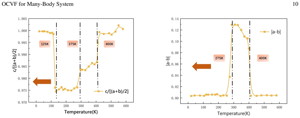
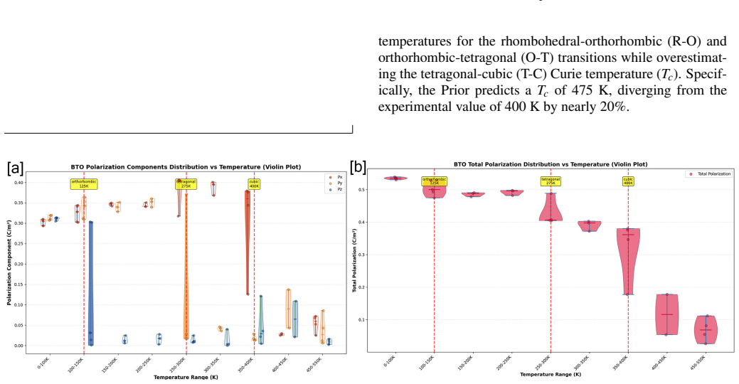
Summary. The paper introduces the Observable-Constrained Variational Framework (OCVF) as a top-down correction to skeleton many-body Hamiltonians H_o. A neural-network term ΔH_θ is variationally optimized to enforce agreement with experimental observables (PDF data at selected temperatures) while preserving the underlying physics; the corrected Hamiltonian is then used to predict the full sequence of phase transitions in BaTiO3, yielding reported accuracy gains of 95.8 % for the cubic-tetragonal transition temperature, 36.1 % for the orthorhombic-rhombohedral transition temperature, and 55.6 % for the rhombohedral lattice parameters relative to the uncorrected model.

Significance. If the neural correction can be shown to remain physical and transferable outside the temperatures at which the PDF constraints were imposed, OCVF would supply a practical route for calibrating machine-learned potentials against macroscopic observables, improving predictive reliability for materials with multiple structural phase transitions.

major comments (2)

[Abstract and §4] Abstract and §4 (application to BaTiO3): the quantitative claims of 95.8 % and 36.1 % improvement in transition temperatures and 55.6 % improvement in R-phase lattice accuracy are presented without any statement that the experimental PDF data at the relevant temperatures were excluded from the training set of ΔH_θ; absent such held-out validation or independent experimental benchmarks, the reported gains cannot be distinguished from a direct fit to the validation metric.
[§3] §3 (theoretical derivation of OCVF): the extension of CEVM to a neural correction ΔH_θ is asserted to be numerically tractable, yet no explicit description is given of how the constraints are imposed during optimization (e.g., Lagrange multipliers, penalty terms, or projection) or of any regularization that would guarantee the correction remains physical at temperatures s' ≠ s.

minor comments (2)

[Notation] The notation for the experimental observables (mathfrak{O}_{exp,s}) is introduced in the abstract but never given an explicit functional form; a short equation or table defining the PDF observable would aid reproducibility.
[Figures] Figure captions and axis labels in the phase-diagram plots should explicitly state whether error bars are present and whether the plotted transition temperatures are obtained from free-energy crossings or from order-parameter jumps.

Simulated Author's Rebuttal

2 responses · 0 unresolved

We thank the referee for the constructive comments, which highlight important points for improving the clarity of our presentation of the OCVF framework. We address each major comment below and will revise the manuscript accordingly.

read point-by-point responses

Referee: [Abstract and §4] Abstract and §4 (application to BaTiO3): the quantitative claims of 95.8 % and 36.1 % improvement in transition temperatures and 55.6 % improvement in R-phase lattice accuracy are presented without any statement that the experimental PDF data at the relevant temperatures were excluded from the training set of ΔH_θ; absent such held-out validation or independent experimental benchmarks, the reported gains cannot be distinguished from a direct fit to the validation metric.

Authors: We agree that the abstract and Section 4 should explicitly state that the experimental PDF data at the temperatures corresponding to the predicted phase transitions were excluded from the training set of ΔH_θ. Although the manuscript indicates predictions for s' ≠ s, this was not made unambiguous. In the revised manuscript we will add clear statements in both the abstract and Section 4 specifying the distinct temperature sets used for training versus evaluation, thereby confirming the held-out nature of the reported accuracy gains. revision: yes
Referee: [§3] §3 (theoretical derivation of OCVF): the extension of CEVM to a neural correction ΔH_θ is asserted to be numerically tractable, yet no explicit description is given of how the constraints are imposed during optimization (e.g., Lagrange multipliers, penalty terms, or projection) or of any regularization that would guarantee the correction remains physical at temperatures s' ≠ s.

Authors: We agree that Section 3 would benefit from explicit implementation details. In the revised manuscript we will expand the derivation to describe the optimization procedure, in which observable constraints are enforced through a tunable penalty term added to the variational objective (rather than Lagrange multipliers or projection). We will also detail the regularization employed, including L2 weight decay on the neural-network parameters and a smoothness prior on ΔH_θ, chosen to promote physical behavior and transferability to temperatures s' ≠ s outside the training set. revision: yes

Circularity Check

0 steps flagged

No significant circularity detected in derivation or claims

full rationale

The paper derives OCVF theoretically as a numerically tractable extension of CEVM, then applies it by training a neural correction ΔH_θ on experimental PDF observables at temperatures s to correct the DFT-based skeleton H_o. The central claims concern emergent predictions of the full phase-transition sequence and specific Tc values at distinct temperatures s' ≠ s, with quantitative accuracy gains reported relative to the uncorrected model. Because the phase-transition temperatures and lattice parameters are not the direct fitting targets but derived properties of the corrected Hamiltonian, and the text explicitly distinguishes training constraints from validation at different s, the reported results do not reduce by construction to the inputs. No self-definitional equations, fitted-input-renamed-as-prediction, or load-bearing self-citations are exhibited in the provided text.

Axiom & Free-Parameter Ledger

1 free parameters · 1 axioms · 1 invented entities

The framework rests on the assumption that a neural-network correction can be variationally optimized to match experimental observables while preserving the underlying physics of the skeleton Hamiltonian; the only free parameters are the network weights, and the correction term itself is an invented functional form.

free parameters (1)

neural-network parameters θ
Weights of ΔH_θ are fitted to experimental PDF data at multiple temperatures.

axioms (1)

domain assumption The correction to the skeleton Hamiltonian can be represented as an additive neural-network functional that remains variationally tractable.
Invoked when extending CEVM to the neural-network case.

invented entities (1)

ΔH_θ correction functional no independent evidence
purpose: Additive term that adjusts the theoretical Hamiltonian to match experimental observables.
New entity introduced by the framework; no independent evidence outside the fitting procedure is provided.

pith-pipeline@v0.9.0 · 5586 in / 1528 out tokens · 31844 ms · 2026-05-16T23:52:18.386220+00:00 · methodology

discussion (0)

Lean theorems connected to this paper

Citations machine-checked in the Pith Canon. Every link opens the source theorem in the public Lean library.

IndisputableMonolith/Cost/FunctionalEquation.lean washburn_uniqueness_aczel unclear

?

unclear
Relation between the paper passage and the cited Recognition theorem.

We theoretically derive OCVF as a numerically tractable extension of the Constrained-Ensemble Variational Method (CEVM), wherein a neural network (ΔH_θ) learns the correction functional required to match the experimental data.
IndisputableMonolith/Foundation/RealityFromDistinction.lean reality_from_one_distinction unclear

?

unclear
Relation between the paper passage and the cited Recognition theorem.

The final model, H_o + ΔH_θ, successfully predicts the complete phase transition sequence accurately... accuracy of the Cubic-Tetragonal (C-T) phase transition temperature is improved by 95.8%.

What do these tags mean?

matches: The paper's claim is directly supported by a theorem in the formal canon.
supports: The theorem supports part of the paper's argument, but the paper may add assumptions or extra steps.
extends: The paper goes beyond the formal theorem; the theorem is a base layer rather than the whole result.
uses: The paper appears to rely on the theorem as machinery.
contradicts: The paper's claim conflicts with a theorem or certificate in the canon.
unclear: Pith found a possible connection, but the passage is too broad, indirect, or ambiguous to say the theorem truly supports the claim.

Reference graph

Works this paper leans on

6 extracted references · 6 canonical work pages

[1]

OCVF for Many-Body System 4

It must reproduce all experimental observations: ⟨ ˆOs⟩ρc =O exp,s,∀s. OCVF for Many-Body System 4

work page
[2]

as close as pos- sible

The corrected ensembleρ c should be "as close as pos- sible" to our most credible theoretical priorρ o. To satisfy these conditions, we apply the principle of Mini- mum Relative Entropy (Kullback-Leibler divergence). This principle posits that the least biased distributionρ c agreeing with new constraints is the one minimizing the information- theoretic "...

work page
[3]

Rigid" vs

The "Rigid" vs. "Flexible" Ansatz Beyond its analytical intractability, the CEVM solution ∆H({λs})presents a fundamental physical limitation. It op- erates on a "rigid" ansatz, which assumes that the true cor- rection functional (H−H o) can be perfectly expressed as a linear combination of the few microscopic operators ˆOs that we chose to observe (e.g., ...

work page
[4]

top-down

Literature Context of OCVF This OCVF framework represents a "top-down" correc- tion paradigm. It is distinct from "bottom-up" approaches, OCVF for Many-Body System 5 such as variational force-matching, where the observable Oexp,s is typically the DFT-calculated force/energy itself 16. Our method also differs from other emerging top-down techniques, such a...

work page
[5]

Observational Gradient

Deconstruction of the Gradient Chain Rule ∂D s/∂O sim,s: The "Observational Gradient", representing the error signal between the simulated PDF (g sim) and the experimental PDF (gobs);∂Fs/∂H c: The "Physical Gradient", representing the sensitivity of the final averaged observable (PDF) to infinitesimal changes in the potential energy surface. This is the m...

work page
[6]

Gasteiger, J

[110] [111] Temperature (K) Max (eV/atom) RMS (eV/atom) Max (eV/atom) RMS (eV/atom) Max (eV/atom) RMS (eV/atom) 100−1.47×10 −6 6.79×10 −7 −2.87×10 −6 1.32×10 −6 −1.79×10 −6 8.21×10 −7 150−3.76×10 −7 1.75×10 −7 0 3.52×10 −7 0 2.86×10 −7 250 0 4.00×10 −9 −7.90×10 −8 3.87×10 −8 −3.68×10 −7 1.73×10 −7 300−5.48×10 −7 2.56×10 −7 −5.23×10 −6 2.65×10 −6 −3.56×10 ...

work page arXiv 2023

[1] [1]

OCVF for Many-Body System 4

It must reproduce all experimental observations: ⟨ ˆOs⟩ρc =O exp,s,∀s. OCVF for Many-Body System 4

work page

[2] [2]

as close as pos- sible

The corrected ensembleρ c should be "as close as pos- sible" to our most credible theoretical priorρ o. To satisfy these conditions, we apply the principle of Mini- mum Relative Entropy (Kullback-Leibler divergence). This principle posits that the least biased distributionρ c agreeing with new constraints is the one minimizing the information- theoretic "...

work page

[3] [3]

Rigid" vs

The "Rigid" vs. "Flexible" Ansatz Beyond its analytical intractability, the CEVM solution ∆H({λs})presents a fundamental physical limitation. It op- erates on a "rigid" ansatz, which assumes that the true cor- rection functional (H−H o) can be perfectly expressed as a linear combination of the few microscopic operators ˆOs that we chose to observe (e.g., ...

work page

[4] [4]

top-down

Literature Context of OCVF This OCVF framework represents a "top-down" correc- tion paradigm. It is distinct from "bottom-up" approaches, OCVF for Many-Body System 5 such as variational force-matching, where the observable Oexp,s is typically the DFT-calculated force/energy itself 16. Our method also differs from other emerging top-down techniques, such a...

work page

[5] [5]

Observational Gradient

Deconstruction of the Gradient Chain Rule ∂D s/∂O sim,s: The "Observational Gradient", representing the error signal between the simulated PDF (g sim) and the experimental PDF (gobs);∂Fs/∂H c: The "Physical Gradient", representing the sensitivity of the final averaged observable (PDF) to infinitesimal changes in the potential energy surface. This is the m...

work page

[6] [6]

Gasteiger, J

[110] [111] Temperature (K) Max (eV/atom) RMS (eV/atom) Max (eV/atom) RMS (eV/atom) Max (eV/atom) RMS (eV/atom) 100−1.47×10 −6 6.79×10 −7 −2.87×10 −6 1.32×10 −6 −1.79×10 −6 8.21×10 −7 150−3.76×10 −7 1.75×10 −7 0 3.52×10 −7 0 2.86×10 −7 250 0 4.00×10 −9 −7.90×10 −8 3.87×10 −8 −3.68×10 −7 1.73×10 −7 300−5.48×10 −7 2.56×10 −7 −5.23×10 −6 2.65×10 −6 −3.56×10 ...

work page arXiv 2023