Aliasing and phase shifting in pseudo-spectral simulations of the incompressible Navier-Stokes equations
Pith reviewed 2026-05-15 13:16 UTC · model grok-4.3
The pith
Phase-shifting dealiasing replaces the 2/3 truncation rule in pseudo-spectral Navier-Stokes simulations and delivers up to threefold speedups at comparable accuracy.
A machine-rendered reading of the paper's core claim, the machinery that carries it, and where it could break.
Core claim
Phase-shifting methods cancel aliasing contributions from quadratic nonlinearities in discrete Fourier space by evaluating nonlinear terms on shifted grids. Depending on the time-stepping scheme, the cancellation is exact or approximate. When applied to the incompressible Navier-Stokes equations, these methods allow the same physical resolution to be achieved on a coarser numerical grid than the conventional 2/3 truncation rule, producing speedups of up to a factor of three at comparable accuracy on the transition of Taylor-Green vortices and forced isotropic turbulence at Re_lambda = 200.
What carries the argument
Phase-shifting dealiasing, in which the nonlinear terms are computed on grids shifted by fractions of the mesh spacing and then linearly combined to remove aliasing errors.
If this is right
- The same maximum wavenumber can be retained while using a grid whose linear size is only two-thirds that demanded by conventional dealiasing.
- Memory footprint and operation count drop proportionally, producing measured speedups of up to three times relative to RK4 with 2/3 truncation.
- The cancellation works with both exact and approximate time integrators, including extensions to forced flows.
- An open-source implementation removes the previous barrier to adoption in existing pseudo-spectral codes.
Where Pith is reading between the lines
- Higher-Reynolds-number direct numerical simulations become feasible on the same hardware because each grid point now carries a larger fraction of the resolved spectrum.
- The shift-and-combine procedure may be combined with other cost-reduction techniques such as adaptive mesh refinement or mixed-precision arithmetic.
- The interaction of phase-shifting with different three-dimensional truncation geometries remains to be mapped systematically beyond the cases tested.
Load-bearing premise
Phase-shifting exactly or approximately cancels the aliasing contributions that arise from quadratic nonlinearities when the nonlinear terms are evaluated on appropriately shifted grids.
What would settle it
A direct comparison of energy spectra or transition times between a phase-shifting run and a standard 2/3-truncation run at the identical maximum wavenumber that shows large, systematic discrepancies.
Figures


read the original abstract
Pseudo-spectral methods are widely used for direct numerical simulations of turbulence, but the standard 2/3 truncation rule for dealiasing is computationally expensive -- accounting for up to 80% of the total cost in three dimensions. Phase shifting methods provide a more efficient alternative by canceling aliasing errors the combination of nonlinear terms evaluated on shifted grids, allowing the same physical resolution to be achieved on a coarser numerical grid. Despite their use in high-resolution turbulence codes, these methods remain poorly documented in the literature and no open-source implementation exists. This paper presents a comprehensive analysis of phase-shifting dealiasing for pseudo-spectral simulations of the incompressible Navier-Stokes equations. We derive the aliasing mechanism from quadratic nonlinearities in discrete Fourier space and explain how phase-shifting cancels aliasing contributions exactly or approximately depending on the time-stepping scheme. We describe and compare several algorithms -- including the exact and approximate RK2 phase-shifting schemes of Patterson Jr and Orszag (1971) and Rogallo (1981), and an extension to forced flows -- and discuss their interaction with different truncation geometries in three dimensions. All algorithms are implemented in the open-source framework Fluidsim, providing the first publicly available implementation of phase-shifting dealiasing for pseudo spectral Navier-Stokes solvers. We evaluate the methods on two test cases: the transition to turbulence of Taylor-Green vortices and forced homogeneous isotropic turbulence at $Re_\lambda = 200$. Phase-shifting methods achieve speedups of up to a factor of 3 compared to RK4 with 2/3 truncation at the same maximum wavenumber, with small accuracy loss.
Editorial analysis
A structured set of objections, weighed in public.
Referee Report
Summary. The manuscript derives the aliasing mechanism for quadratic nonlinearities in discrete Fourier space for pseudo-spectral incompressible Navier-Stokes simulations. It shows how phase-shifting on shifted grids cancels aliasing contributions exactly for the Patterson-Orszag RK2 scheme and approximately for other schemes such as Rogallo's, extends the approach to forced flows and 3D truncation geometries, implements all variants in the open-source Fluidsim framework, and reports quantitative benchmarks on Taylor-Green vortex transition and forced HIT at Re_λ=200. The central claim is that phase-shifting achieves up to 3× speedup versus RK4+2/3 truncation at fixed k_max with only small accuracy loss.
Significance. If the derivation and numerical results hold, the work is significant because it supplies the first publicly available open-source implementation of phase-shifting dealiasing together with a self-contained analytic treatment and reproducible benchmarks on two standard test cases. The reported factor-of-3 speedup directly addresses the dominant cost of the 2/3 rule (up to 80 % of runtime in 3D) while preserving the same maximum wavenumber, and the explicit treatment of truncation geometries and forced-flow extensions fills a documented gap in the literature.
minor comments (2)
- [Abstract and §4] The abstract and introduction state that phase-shifting yields 'small accuracy loss,' but the quantitative error metrics (e.g., kinetic-energy spectra or enstrophy) and their comparison to the 2/3-rule baseline are only summarized; a short table or explicit statement of the observed relative errors at equivalent k_max would strengthen the claim.
- [Section on truncation geometries] In the discussion of 3D truncation geometries, the interaction between the phase-shift vectors and the spherical versus cubic cutoff is described but not illustrated; a single schematic diagram showing the shifted wavenumber supports would improve clarity for readers implementing the method.
Simulated Author's Rebuttal
We thank the referee for the detailed summary, positive significance assessment, and recommendation of minor revision. No specific major comments were listed in the report, so we have no points to address point-by-point at this stage. We will incorporate any minor editorial or clarification changes suggested during the revision process.
Circularity Check
Derivation self-contained; no circular reductions identified
full rationale
The paper derives aliasing directly from quadratic nonlinearities in discrete Fourier space using standard properties of the discrete Fourier transform, then shows exact or approximate cancellation under phase-shifting for specific time-stepping schemes (Patterson-Orszag RK2, Rogallo). These steps rely on explicit algebraic manipulation of convolution terms rather than any fitted parameter or self-referential definition. Prior schemes are cited from independent 1971/1981 literature with no author overlap, and the central speedup claim (factor ~3 at fixed k_max) is obtained from explicit numerical benchmarks on Taylor-Green transition and Re_λ=200 HIT, not from any prediction that reduces to the input data by construction. The open-source Fluidsim implementation supplies reproducible code, confirming the analysis is externally falsifiable and independent of the present paper's fitted values or self-citations.
Axiom & Free-Parameter Ledger
axioms (2)
- domain assumption Incompressible Navier-Stokes equations expressed in Fourier space
- standard math Quadratic nonlinearities produce aliasing via discrete Fourier convolution
Reference graph
Works this paper leans on
-
[1]
General description We consider equations that can be written in spectral space as: ∂tS=σS+N(S),(16) whereSrepresents the state of the system (potentially containing several variables),σ(k) is a real or complex coefficient depending on the wavenumber, andN(S) is an operator with at most second-order nonlinearities. The incompressible Navier-Stokes equatio...
-
[2]
Application to the quadratic 1D model We first use the one-dimensional (1D) model defined by Eq. (11) to verify the behavior of the different algorithms and our implementations. Fig. 7 displays the maximum of|S(k, dt)− Sexact(k, dt)|as a function of the time stepdtfor standard schemes (Euler, RK2, and RK4) and for the two RK2 phase-shifting schemes descri...
-
[3]
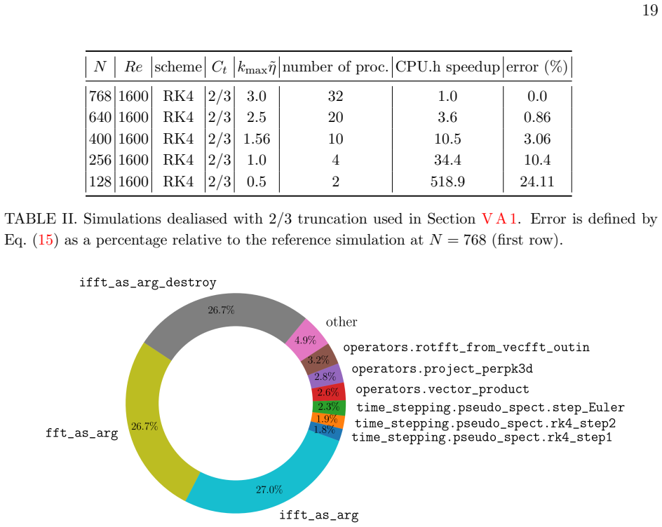
Effect of resolution for RK4 truncated simulations We consider simulations dealiased with 2/3 truncation at four grid sizes:N= 128, 256, 400, 640, and 768 (Table II). Since we compare resolutions, these simulations are run in parallel with a reasonable number of cores for each grid size. 19 N Re scheme Ct kmax˜ηnumber of proc. CPU.h speedup error (%) 768 ...
-
[4]
We already studied in Section III D how aliasing errors affect a simulation at smallk max˜η= 0.75
Effect ofk max˜ηon aliasing error Having quantified the effect of resolution on fully dealiased simulations, we now examine how resolution affects aliasing errors. We already studied in Section III D how aliasing errors affect a simulation at smallk max˜η= 0.75. Here, we consider analogous simulations but for kmax˜η >3 (see Table III). Fig. 14 shows the e...
-
[5]
Profiles and speedup We profile the different algorithms implemented in Fluidsim on short Taylor-Green simu- lations as described in Section III D, focusing on time-stepping performance. To isolate the effect of the time-stepping algorithm, we always compare in this subsection simulations run with the same number of cores. Fig. 16 compares the distributio...
-
[6]
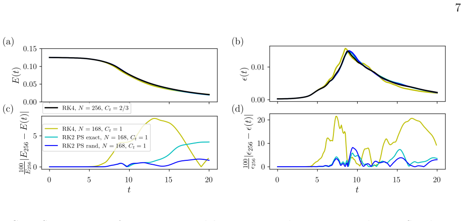
Effect of time scheme and Reynolds number We now present three series of four simulations each, listed in Table IV. The three series correspond to different (Re, k max˜η) combinations: (1600,1), (2800,0.6), and (1600,1.6). Each series consists of four simulations: a reference run with the RK4 scheme andC t = 2/3; a second RK4 run withC t = 1; and two runs...
-
[7]
Quality and speedup To generalize the conclusions of the previous section, we explore whether intermediate combinations of truncation and phase shifting can improve the compromise between speedup and accuracy. Because the speedup trends appear to be independent ofk max, we fixk max = 108 (kmax˜η≈1.27) and compare all combinations of time scheme and trunca...
work page 2020
-
[10]
A. Delache, C. Cambon, and F. Godeferd, Scale by scale anisotropy in freely decaying rotating turbulence, Physics of Fluids26, 025104 (2014)
work page 2014
-
[12]
K. P. Iyer, K. R. Sreenivasan, and P. Yeung, Circulation in high Reynolds number isotropic turbulence is a bifractal, Physical Review X9, 041006 (2019)
work page 2019
- [13]
-
[15]
K. J. Burns, G. M. Vasil, J. S. Oishi, D. Lecoanet, and B. P. Brown, Dedalus: A flexible framework for numerical simulations with spectral methods, Physical Review Research2, 023068 (2020)
work page 2020
-
[16]
P. D. Mininni, D. Rosenberg, R. Reddy, and A. Pouquet, A hybrid MPI–OpenMP scheme for scalable parallel pseudospectral computations for fluid turbulence, Parallel Computing37, 316 (2011)
work page 2011
-
[17]
M. Mortensen and H. P. Langtangen, High performance Python for direct numerical simula- tions of turbulent flows, Computer Physics Communications203, 53 (2016)
work page 2016
-
[18]
C. C. Lalescu, B. Bramas, M. Rampp, and M. Wilczek, An efficient particle tracking algo- rithm for large-scale parallel pseudo-spectral simulations of turbulence, Computer Physics Communications278, 108406 (2022)
work page 2022
-
[19]
S. G. Chumakov, A priori study of subgrid-scale flux of a passive scalar in isotropic homoge- neous turbulence, Physical Review E78, 036313 (2008)
work page 2008
-
[20]
A. V. Mohanan, C. Bonamy, M. C. Linares, and P. Augier, FluidSim: Modular, object-oriented Python package for high-performance CFD simulations, Journal of Open Research Software 7, 10.5334/jors.239 (2019)
-
[21]
C. Lambert, J. Reneuve, and P. Augier, Dataset for article ”aliasing and phase shifting in pseudo-spectral simulations of the incompressible navier-stokes equations”, 10.5281/zen- odo.19554006 (2026). 34
-
[22]
G. I. Taylor and A. E. Green, Mechanism of the production of small eddies from large ones, Proceedings of the Royal Society of London. Series A, Mathematical and Physical Sciences 158, 499 (1937)
work page 1937
-
[24]
The documentation for this module is available in the Fluidsim documentation at https://fluidsim.readthedocs.io/en/latest/generated/fluidsim.base.time_ stepping.pseudo_spect.html
-
[25]
See Supplemental Material at URL-will-be-inserted-by-publisher
-
[26]
J. R. Debonis, Solutions of the Taylor-Green vortex problem using high-resolution explicit finite difference methods (2013). [20]https://fluidsim.readthedocs.io/en/latest/generated/fluidsim.base.time_ stepping.pseudo_spect.html
work page 2013
-
[27]
V. Eswaran and S. Pope, An examination of forcing in direct numerical simulations of turbu- lence, Computers & Fluids16, 257 (1988). Supplementary material: Aliasing and phase shifting in pseudo-spectral simulations of the incompressible Navier-Stokes equations Clovis Lambert, 1 Jason Reneuve, 1 and Pierre Augier 1,∗ 1Laboratoire des Ecoulements G´ eophys...
work page 1988
- [28]
- [29]
-
[30]
J. Cooley and J. Tukey, An algorithm for the machine calculation of complex Fourier series, Mathematics of Computation19, 297 (1965)
work page 1965
-
[31]
A. V. Mohanan, C. Bonamy, and P. Augier, FluidFFT: Common API (C++ and Python) for Fast Fourier Transform HPC libraries, Journal of Open Research Software7, 10.5334/jors.238 (2019)
-
[32]
L. Carleson, On convergence and growth of partial sums of fourier series, Acta Mathematica 116, 135 (1966). 9
work page 1966
-
[33]
O. H. Hald, Convergence of Fourier methods for Navier-Stokes equations, Journal of Compu- tational Physics40, 305 (1981)
work page 1981
-
[34]
G. Patterson Jr and S. A. Orszag, Spectral calculations of isotropic turbulence: Efficient removal of aliasing interactions, The Physics of Fluids14, 2538 (1971)
work page 1971
-
[35]
R. S. Rogallo,Numerical experiments in homogeneous turbulence, Vol. 81315 (National Aero- nautics and Space Administration, 1981)
work page 1981
discussion (0)
Sign in with ORCID, Apple, or X to comment. Anyone can read and Pith papers without signing in.