Breakthrough the Suboptimal Stable Point in Value-Factorization-Based Multi-Agent Reinforcement Learning
Pith reviewed 2026-05-10 19:57 UTC · model grok-4.3
The pith
Non-optimal stable points primarily cause value-factorization multi-agent reinforcement learning to converge to suboptimal solutions.
A machine-rendered reading of the paper's core claim, the machinery that carries it, and where it could break.
Core claim
The paper claims that non-optimal stable points are the primary cause of poor performance in value-factorization-based multi-agent reinforcement learning. Existing methods contain distributions rich in such points. Making the optimal action the unique stable point is nearly infeasible, whereas iteratively filtering suboptimal actions by rendering them unstable offers a practical route to global optimality. The Multi-Round Value Factorization framework realizes this by measuring a non-negative payoff increment relative to the previously selected action, thereby transforming inferior actions into unstable points and driving each iteration toward a stable point with a superior action.
What carries the argument
The stable point, which characterizes the potential convergence targets of value factorization in general cases, together with the iterative filtering mechanism that uses non-negative payoff increments to destabilize inferior actions.
If this is right
- Non-optimal stable points explain the performance gaps observed in current value-factorization methods.
- Iteratively rendering suboptimal actions unstable is a feasible route to global optimality.
- The Multi-Round Value Factorization framework implements this filtering via payoff increments relative to prior actions.
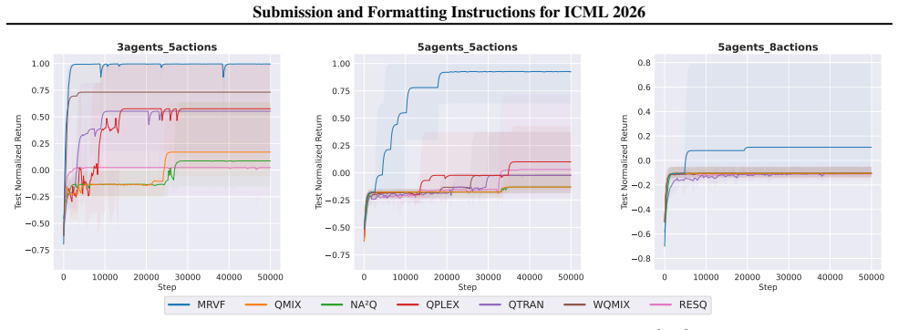
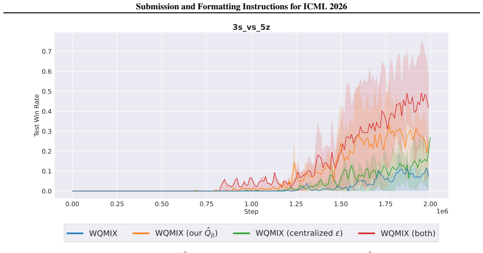
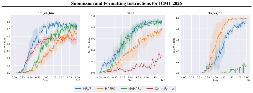
- Experiments on predator-prey tasks and the StarCraft II Multi-Agent Challenge confirm both the stable-point analysis and improved performance over prior methods.
Where Pith is reading between the lines
- The stable-point lens could be used to audit convergence behavior in other multi-agent algorithms that rely on value decomposition.
- Similar iterative destabilization of inferior choices might transfer to single-agent reinforcement learning settings that employ factored value functions.
- In deployed multi-agent systems such as robotic teams, injecting controlled instability at each round could reduce the frequency of coordinated but inefficient behaviors.
Load-bearing premise
A non-negative payoff increment measured relative to the previously selected action can reliably transform inferior actions into unstable points without creating new suboptimal stable points or disrupting overall convergence properties.
What would settle it
Applying the Multi-Round Value Factorization framework to the StarCraft II Multi-Agent Challenge benchmark and finding that it still converges to the same suboptimal policies identified in the stable-point analysis of baseline methods would falsify the claim.
Figures


read the original abstract
Value factorization, a popular paradigm in MARL, faces significant theoretical and algorithmic bottlenecks: its tendency to converge to suboptimal solutions remains poorly understood and unsolved. Theoretically, existing analyses fail to explain this due to their primary focus on the optimal case. To bridge this gap, we introduce a novel theoretical concept: the stable point, which characterizes the potential convergence of value factorization in general cases. Through an analysis of stable point distributions in existing methods, we reveal that non-optimal stable points are the primary cause of poor performance. However, algorithmically, making the optimal action the unique stable point is nearly infeasible. In contrast, iteratively filtering suboptimal actions by rendering them unstable emerges as a more practical approach for global optimality. Inspired by this, we propose a novel Multi-Round Value Factorization (MRVF) framework. Specifically, by measuring a non-negative payoff increment relative to the previously selected action, MRVF transforms inferior actions into unstable points, thereby driving each iteration toward a stable point with a superior action. Experiments on challenging benchmarks, including predator-prey tasks and StarCraft II Multi-Agent Challenge (SMAC), validate our analysis of stable points and demonstrate the superiority of MRVF over state-of-the-art methods.
Editorial analysis
A structured set of objections, weighed in public.
Referee Report
Summary. The paper claims that value factorization in MARL tends to converge to suboptimal solutions because of non-optimal 'stable points,' a new concept characterizing general convergence behavior beyond the optimal case. Analysis of stable point distributions in existing methods identifies these as the primary cause of poor performance. The authors propose the Multi-Round Value Factorization (MRVF) framework, which iteratively adds a non-negative payoff increment relative to the previously selected action to render inferior actions unstable, thereby driving each round toward a stable point with a superior action. Experiments on predator-prey tasks and SMAC benchmarks are said to validate the stable-point analysis and show MRVF outperforming state-of-the-art methods.
Significance. If the stable-point characterization is shown to be independent of the value factorization and the MRVF increment provably eliminates suboptimal attractors without introducing new ones or violating convergence, the work would offer a useful theoretical lens on a persistent MARL bottleneck and a practical algorithmic fix. The empirical validation on SMAC provides some evidence of utility, but the absence of parameter-free derivations or machine-checked proofs limits the strength of the contribution relative to prior fixed-point analyses in RL.
major comments (3)
- [§3] §3 (stable point definition and distribution analysis): the stable point is introduced as a novel construct without an explicit derivation showing it reduces to or is independent of the standard fixed-point condition of value factorization; this creates a circularity risk because the MRVF payoff increment is itself defined relative to the learned values.
- [§4] §4 (MRVF mechanism): no derivation is supplied showing how the non-negative payoff increment modifies the fixed-point equation to destabilize suboptimal actions globally; the claim that this process cannot create fresh suboptimal stable points or break overall convergence therefore lacks support and is load-bearing for the central algorithmic claim.
- [§5] §5 (experiments): the reported results on SMAC and predator-prey lack ablations isolating the effect of the payoff increment on stable-point distributions across rounds; without these, it is impossible to confirm that performance gains arise from the proposed filtering rather than hyperparameter tuning or other implementation details.
minor comments (2)
- [Abstract] Abstract and §2: the phrase 'analysis of stable point distributions' is used without specifying the quantitative metrics or visualization methods employed.
- [§4] Notation: the payoff increment is described as 'non-negative' but its precise functional form and dependence on the value function are not clarified in the high-level description.
Simulated Author's Rebuttal
We thank the referee for the insightful and constructive comments. We address each major comment point by point below, indicating where revisions will be made and providing honest clarifications on the theoretical aspects.
read point-by-point responses
-
Referee: [§3] §3 (stable point definition and distribution analysis): the stable point is introduced as a novel construct without an explicit derivation showing it reduces to or is independent of the standard fixed-point condition of value factorization; this creates a circularity risk because the MRVF payoff increment is itself defined relative to the learned values.
Authors: We appreciate this observation on the need for clearer grounding. The stable point is defined in §3 as the action a satisfying Q(s, a) = max_{a'} Q(s, a') under the factorization operator, which directly generalizes the standard fixed-point for the optimal case. In the revision we will insert an explicit derivation in §3.1 showing that the condition reduces exactly to the Bellman fixed-point equation when a is optimal, while for suboptimal actions it identifies local attractors where the equality holds without global maximality. This derivation relies only on the learned Q-values from any value factorization method and is therefore independent of the subsequent MRVF increment. The increment is applied only after the base factorization has converged, to modify the effective payoff landscape for the next round; we will add a sentence clarifying that the stable-point definition itself does not depend on MRVF. revision: partial
-
Referee: [§4] §4 (MRVF mechanism): no derivation is supplied showing how the non-negative payoff increment modifies the fixed-point equation to destabilize suboptimal actions globally; the claim that this process cannot create fresh suboptimal stable points or break overall convergence therefore lacks support and is load-bearing for the central algorithmic claim.
Authors: We acknowledge that the current manuscript offers an intuitive description rather than a formal derivation of how the increment alters the fixed-point equation. In the revision we will add a short mathematical sketch in §4.2: for an inferior action a, the update sets an effective Q'(s, a) = Q(s, a) + δ (δ > 0 chosen as the gap to the superior action), which violates the stability equality Q(s, a) = max Q(s, ·) and thereby renders a unstable. This forces the next round to converge to a stable point with a strictly better action. However, a complete global guarantee that no new suboptimal stable points can arise or that convergence is preserved in every environment would require additional assumptions (e.g., Lipschitz continuity of the value functions and bounded increments) that are not established in the present work. We will therefore present the sketch as supporting analysis, note the limitation explicitly, and rely on the empirical evidence that the procedure converges reliably on the tested domains. revision: partial
-
Referee: [§5] §5 (experiments): the reported results on SMAC and predator-prey lack ablations isolating the effect of the payoff increment on stable-point distributions across rounds; without these, it is impossible to confirm that performance gains arise from the proposed filtering rather than hyperparameter tuning or other implementation details.
Authors: We agree that stronger isolation of the increment mechanism is necessary. In the revised §5 we will add two sets of results: (1) histograms of stable-point quality (optimal vs. suboptimal) measured at the end of each MRVF round on both predator-prey and SMAC maps, and (2) a controlled ablation in which the increment δ is set to zero while all other hyperparameters and network architectures remain identical. These additions will directly demonstrate that the observed performance lift originates from the iterative destabilization of inferior actions rather than from incidental hyperparameter effects. revision: yes
- A complete machine-checked or parameter-free proof that MRVF cannot introduce new suboptimal stable points in arbitrary environments.
Circularity Check
No significant circularity detected
full rationale
The abstract introduces the novel concept of a 'stable point' to characterize general convergence behavior of value factorization (beyond optimal cases only), analyzes distributions of these points in existing methods to identify non-optimal ones as the primary cause of suboptimality, and proposes MRVF as an iterative filtering approach using a non-negative payoff increment. No equations, self-citations, or fitted parameters are exhibited that reduce the central claims, the definition of stable points, or the MRVF mechanism to prior inputs by construction. The derivation chain relies on the independent theoretical construct and external benchmark validation, remaining self-contained.
Axiom & Free-Parameter Ledger
axioms (2)
- domain assumption Value factorization methods converge to stable points characterized by individual agent action stability in general cases.
- ad hoc to paper A non-negative payoff increment relative to the prior action can be used to identify and destabilize inferior actions.
invented entities (1)
-
stable point
no independent evidence
Reference graph
Works this paper leans on
-
[1]
¯u̸= eu Here we give a specificQ mon that satisfies these conditions: Qmon(τ,u) = ( Qjt(τ,eu)u= eu maxu Qjt(τ,u) + ∆otherwise (32) where ∆>0 . We let Qr =Q jt −Q mon. Since Qmon ≥Q jt, we have Qr ≤0 . Therefore, we obtain Qmon, wr and Qr, which together constitute theQ tot of ResQ. ∀u̸= eu, we have Qjt(τ,u) =Q tot(τ,u) =Q mon(τ,u) + 1∗Q r(τ,u) . Foreu, si...
work page 2022
-
[2]
¯u=u ∗ whereQ mon ≡Q jt(τ,u ∗)is a specific case. We let Qr =Q jt −Q mon. Since Qmon ≥Q jt, we have Qr ≤0 . Therefore, we obtain Qmon, wr and Qr, which together constitute theQ tot of ResQ. According tow r defined in Equation (30), we have Qtot = ( Qmon(τ,u) + 1∗Q r(τ,u)∀u̸= eu Qmon(τ,eu) + 0∗Q r(τ,eu)u= eu (33) SubstitutingQ r =Q jt −Q mon andQ mon(τ,eu)...
work page 2026
discussion (0)
Sign in with ORCID, Apple, or X to comment. Anyone can read and Pith papers without signing in.