pith. the verified trust layer for science. sign in

arxiv: 2604.10396 · v1 · submitted 2026-04-12 · 🪐 quant-ph

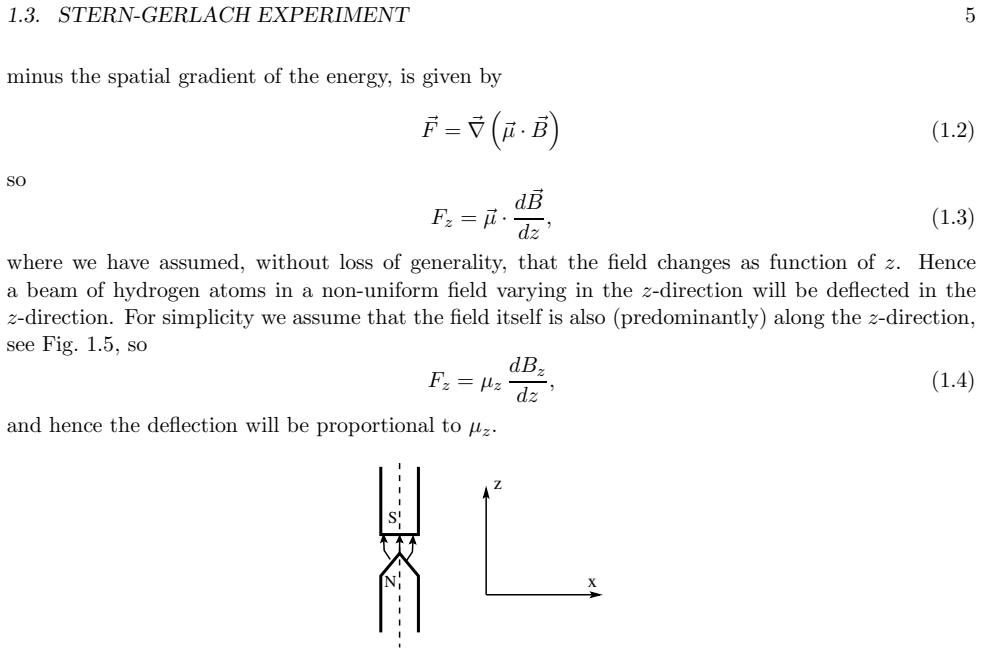
An Undergraduate Course in Quantum Computing

Pith reviewed 2026-05-10 16:47 UTC · model grok-4.3

classification 🪐 quant-ph
keywords quantum computingShor's algorithmquantum error correctionundergraduate courselinear algebraphysical sciencesquantum algorithmspedagogy
0
0 comments X p. Extension

The pith

Quantum computing can be taught to physical sciences undergraduates using only linear algebra as background.

A machine-rendered reading of the paper's core claim, the machinery that carries it, and where it could break.
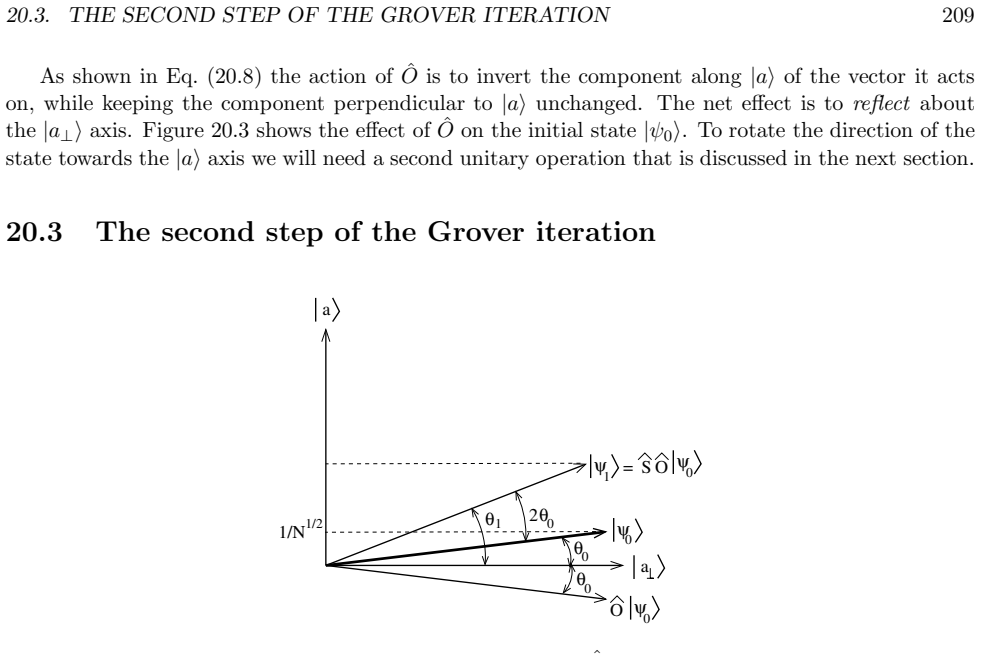
The paper supplies the complete text and materials for a one-quarter or one-semester undergraduate course on quantum computing aimed at students in the physical sciences. It begins with a review of linear algebra and then develops the necessary quantum ideas from the ground up, without assuming any prior quantum mechanics. The course is structured to reach its core topics of Shor's factoring algorithm and an introduction to quantum error correction. A sympathetic reader would care because the approach removes a common prerequisite barrier and makes these advanced subjects reachable in a standard undergraduate setting.

Core claim

This text serves as a complete one quarter or one semester undergraduate course on quantum computing that has been given at the University of California Santa Cruz. It is intended for students in the physical sciences who have already studied linear algebra (though a review of this topic is given in the course). No prior knowledge of quantum mechanics is required. The most important topics covered are Shor's algorithm and an introduction to quantum error correction. Most of the text is a build-up to these topics.

What carries the argument

The progressive curriculum that reviews linear algebra and builds quantum computing concepts step by step to reach Shor's algorithm and quantum error correction.

Load-bearing premise

The material presented in this order from a linear algebra foundation alone enables students to understand and apply Shor's algorithm and quantum error correction.

What would settle it

If a class of target students who complete the course cannot explain the key steps of Shor's algorithm on a follow-up assessment, the claim that the text works as a complete course would be undermined.

Figures

Figures reproduced from arXiv: 2604.10396 by Peter Young.

Figure 1.1
Figure 1.1. Figure 1.1: A beam of light spreads out (diffracts) when passin [PITH_FULL_IMAGE:figures/full_fig_p010_1_1.png] view at source ↗
Figure 1.2
Figure 1.2. Figure 1.2: A two slit experiment. Interference fringes, os [PITH_FULL_IMAGE:figures/full_fig_p010_1_2.png] view at source ↗
Figure 1.3
Figure 1.3. Figure 1.3: The difference in the length of the paths taken by th [PITH_FULL_IMAGE:figures/full_fig_p011_1_3.png] view at source ↗
Figure 1.4
Figure 1.4. Figure 1.4: We record the number of clicks for counters placed a [PITH_FULL_IMAGE:figures/full_fig_p011_1_4.png] view at source ↗
Figure 1.5
Figure 1.5. Figure 1.5: A cross section of the magnet in the Stern-Gerlac [PITH_FULL_IMAGE:figures/full_fig_p013_1_5.png] view at source ↗
Figure 1.6
Figure 1.6. Figure 1.6: The Stern-Gerlach apparatus. We send in a beam of unpolarized hydrogen atoms into a non-uniform field. This is the famous Stern-Gerlach (SG) experiment. Since the direction of ~µ is random, classically µz takes a range of values, so we would expect a continuous range of deflections. However, it is found that only two beams [PITH_FULL_IMAGE:figures/full_fig_p013_1_6.png] view at source ↗
Figure 1.7
Figure 1.7. Figure 1.7: The upper figure shows schematically separate St [PITH_FULL_IMAGE:figures/full_fig_p014_1_7.png] view at source ↗
Figure 1.8
Figure 1.8. Figure 1.8: We now add another SGz apparatus after the SGx apparatus in [PITH_FULL_IMAGE:figures/full_fig_p015_1_8.png] view at source ↗
Figure 4.1
Figure 4.1. Figure 4.1: The Bloch sphere. Note that we can always multiply eigenstates by an arbitrary phase factor so you might see expres￾sions for these eigenstates which look different from Eqs. (4.12a) and (4.12b), but which are actually equivalent. If we consider a point on a unit sphere (often called the Bloch sphere) with polar angles θ and φ, then the eigenstate of spin in that direction with eigenvalue +1 is given by … view at source ↗
Figure 6.1
Figure 6.1. Figure 6.1: Sketch of the experimental setup for the version [PITH_FULL_IMAGE:figures/full_fig_p069_6_1.png] view at source ↗
Figure 6.2
Figure 6.2. Figure 6.2: A possible choice of directions for which the Bel [PITH_FULL_IMAGE:figures/full_fig_p073_6_2.png] view at source ↗
Figure 6
Figure 6. Figure 6: , the inequality in Eq. (6.21) can be written [PITH_FULL_IMAGE:figures/full_fig_p073_6.png] view at source ↗
Figure 6.3
Figure 6.3. Figure 6.3: A graph showing that the inequality in Eq. (6.24) [PITH_FULL_IMAGE:figures/full_fig_p073_6_3.png] view at source ↗
Figure 7.1
Figure 7.1. Figure 7.1: The CNOT gate. The input is on the left and the outp [PITH_FULL_IMAGE:figures/full_fig_p081_7_1.png] view at source ↗
Figure 7.2
Figure 7.2. Figure 7.2: The Toffoli gate. This has two control bits [PITH_FULL_IMAGE:figures/full_fig_p081_7_2.png] view at source ↗
Figure 7.3
Figure 7.3. Figure 7.3: Left: the Fredkin gate. This is a controlled-swa [PITH_FULL_IMAGE:figures/full_fig_p081_7_3.png] view at source ↗
Figure 7.4
Figure 7.4. Figure 7.4: A schematic circuit with three qubits and two gat [PITH_FULL_IMAGE:figures/full_fig_p082_7_4.png] view at source ↗
Figure 7.5
Figure 7.5. Figure 7.5: Two ways of drawing a CNOT gate. The right hand way [PITH_FULL_IMAGE:figures/full_fig_p084_7_5.png] view at source ↗
Figure 7.6
Figure 7.6. Figure 7.6: The action of the CNOT gate when the upper (contro [PITH_FULL_IMAGE:figures/full_fig_p085_7_6.png] view at source ↗
Figure 7
Figure 7. Figure 7: in which there are two CNOTs with opposite orientati [PITH_FULL_IMAGE:figures/full_fig_p085_7.png] view at source ↗
Figure 7.7
Figure 7.7. Figure 7.7: A circuit with 2 CNOTs in opposite orientations. [PITH_FULL_IMAGE:figures/full_fig_p085_7_7.png] view at source ↗
Figure 7.8
Figure 7.8. Figure 7.8: The initial state of both qubits is |0i. What is the final state |ψ3i? Equation (7.16) gives the state of the two qubits at each stage. The end result is that the two qubits are entangled and, in contrast to what one might have thought, the control (upper) qubit has a non-zero amplitude to be flipped relative to its initial state, i.e. to be in state |1i. It is useful to mention here that one has to be c… view at source ↗
Figure 7.9
Figure 7.9. Figure 7.9: A circuit with a control-U gate in which the control (upper) qubit is surrounded by Hadamards. U is an operator with eigenvalues ±1 and corresponding eigenvectors |ψ+i and |ψ−i. As shown in the text, if a measurement of the upper qubit gives |0i then the lower qubit will be in state |ψ+i, and if the measurement gives |1i then the lower qubit will be in state |ψ−i. The states |φii(i = 0, 1, 2, 3) are desc… view at source ↗
Figure 8.1
Figure 8.1. Figure 8.1: Circuit to create the Bell states defined by Eqs. ( [PITH_FULL_IMAGE:figures/full_fig_p091_8_1.png] view at source ↗
Figure 8.2
Figure 8.2. Figure 8.2: Circuit for Bell measurements. This will be used [PITH_FULL_IMAGE:figures/full_fig_p092_8_2.png] view at source ↗
Figure 9.1
Figure 9.1. Figure 9.1: Schematic diagram of a unitary transformation [PITH_FULL_IMAGE:figures/full_fig_p093_9_1.png] view at source ↗
Figure 9.2
Figure 9.2. Figure 9.2: Schematic diagram of a general unitary transfor [PITH_FULL_IMAGE:figures/full_fig_p094_9_2.png] view at source ↗
Figure 9.3
Figure 9.3. Figure 9.3: Because of the Hadamards, the input to Uf is now the uniform superposition of all com￾putational basis states in Eq. (9.6). The output from Uf is given by Eq. (9.9). This is an astonishing result. The final state contains the function values for all 2 n possible values of the input x. They have been evaluated in parallel, a feature of quantum mechanics called, naturally enough, “quantum parallelism”. For… view at source ↗
Figure 10.1
Figure 10.1. Figure 10.1: The blackbox routine Uf for a function f(x) which takes a 1-qubit input x and computes a 1-qubit function f(x). Here x and y are computational basis states |0i or |1i. However, to gain a quantum speedup, we will input superpositions, generated by Hadamard gates, as shown in [PITH_FULL_IMAGE:figures/full_fig_p098_10_1.png] view at source ↗
Figure 10.2
Figure 10.2. Figure 10.2: Circuit for Deutsch’s algorithm. The initial s [PITH_FULL_IMAGE:figures/full_fig_p098_10_2.png] view at source ↗
Figure 10.4
Figure 10.4. Figure 10.4: We now explain each of the diagrams in this figure. • f1: This follows simply because Uf1 makes no change, see [PITH_FULL_IMAGE:figures/full_fig_p100_10_4.png] view at source ↗
Figure 10.3
Figure 10.3. Figure 10.3: Circuit diagrams for each of the four functions [PITH_FULL_IMAGE:figures/full_fig_p101_10_3.png] view at source ↗
Figure 10.4
Figure 10.4. Figure 10.4: This is correct because the function is balanced. [PITH_FULL_IMAGE:figures/full_fig_p101_10_4.png] view at source ↗
Figure 10.4
Figure 10.4. Figure 10.4: The circuits for the four functions f1, · · · , f4 given in [PITH_FULL_IMAGE:figures/full_fig_p102_10_4.png] view at source ↗
Figure 10.5
Figure 10.5. Figure 10.5: Some useful identities in quantum circuits. Of [PITH_FULL_IMAGE:figures/full_fig_p103_10_5.png] view at source ↗
Figure 10
Figure 10. Figure 10: (f)(ii). Now the [PITH_FULL_IMAGE:figures/full_fig_p103_10.png] view at source ↗
Figure 11.1
Figure 11.1. Figure 11.1: Circuit diagram for the Bernstein-Vazirani al [PITH_FULL_IMAGE:figures/full_fig_p106_11_1.png] view at source ↗
Figure 11.2
Figure 11.2. Figure 11.2: A circuit diagram for n = 5 to implement the function f(x) = a · x with a = 11010, i.e. f(x) = x1 ⊕ x3 ⊕ x4. The circuit flips the output qubit, the lowest one, initialized to y, whenever x1 ⊕ x3 ⊕ x4 = 1. (Note that flipping y is equivalent to adding 1 to y mod 2.) Hence the final value of the output qubit is y ⊕ (a · x) = y ⊕ x1 ⊕ x3 ⊕ x4 as required. To incorporate Uf into the Bernstein-Vazirani algo… view at source ↗
Figure 11.3
Figure 11.3. Figure 11.3: Sandwiching the circuit for Uf in [PITH_FULL_IMAGE:figures/full_fig_p108_11_3.png] view at source ↗
Figure 12.1
Figure 12.1. Figure 12.1: Circuit diagram for Simon’s algorithm. The upp [PITH_FULL_IMAGE:figures/full_fig_p114_12_1.png] view at source ↗
Figure 14.1
Figure 14.1. Figure 14.1: The function f(x) ≡ 4 x (mod 91 ). The period is seen by inspection to equal 6. understand how this figure is obtained by working out the values of 4x (mod 91 ) for x = 1, 2, · · · , 6. x = 1, 4 x = 4 , (14.6a) x = 2, 4 x = 16 , (14.6b) x = 3, 4 x = 64 , (14.6c) x = 4, 4 x = 64 × 4 = 256 = 2 × 91 + 74 ≡ 74 ( mod 91 ), (14.6d) x = 5, 4 x ≡ 74 × 4 = 296 = 3 × 91 + 23 ≡ 23 ( mod 91 ), (14.6e) x = 6, 4 x ≡ … view at source ↗
Figure 14.2
Figure 14.2. Figure 14.2: The function f(x) ≡ 19x (mod 91 ). The period is seen by inspection to equal 12. const. pq. Since p and q are primes (and neither a r/2 + 1 nor a r/2 − 1  are multiples of pq), this is only possible if a r/2 + 1 is a multiple of one of the factors, p say, i.e. a r/2 + 1 = Cp, and a r/2−1 is a multiple of the other one q, i.e. a r/2−1 = C ′ q (C and C ′ are constants). Consequently p is the greatest co… view at source ↗
Figure 15.1
Figure 15.1. Figure 15.1 [PITH_FULL_IMAGE:figures/full_fig_p130_15_1.png] view at source ↗
Figure 15.1
Figure 15.1. Figure 15.1: A graphical representation of Eqs. (15.14)–(1 [PITH_FULL_IMAGE:figures/full_fig_p131_15_1.png] view at source ↗
Figure 16.1
Figure 16.1. Figure 16.1: The QFT for one qubit. The output from the Hadama [PITH_FULL_IMAGE:figures/full_fig_p138_16_1.png] view at source ↗
Figure 16.2
Figure 16.2. Figure 16.2: The initial state on the left is the single quant [PITH_FULL_IMAGE:figures/full_fig_p139_16_2.png] view at source ↗
Figure 16.3
Figure 16.3. Figure 16.3: The same as Fig. 16.2 but with the addition of a sw [PITH_FULL_IMAGE:figures/full_fig_p140_16_3.png] view at source ↗
Figure 16.4
Figure 16.4. Figure 16.4: Circuit diagram for performing the QFT with [PITH_FULL_IMAGE:figures/full_fig_p142_16_4.png] view at source ↗
Figure 16.5
Figure 16.5. Figure 16.5: Circuit diagram for performing the QFT with an a [PITH_FULL_IMAGE:figures/full_fig_p143_16_5.png] view at source ↗
Figure 16.6
Figure 16.6. Figure 16.6: The circuit for phase estimation for 1 bit of pre [PITH_FULL_IMAGE:figures/full_fig_p144_16_6.png] view at source ↗
Figure 16.7
Figure 16.7. Figure 16.7: The circuit for phase estimation for two bits of [PITH_FULL_IMAGE:figures/full_fig_p145_16_7.png] view at source ↗
Figure 16.7
Figure 16.7. Figure 16.7: According to Eq. (16.28), the final measurement in [PITH_FULL_IMAGE:figures/full_fig_p146_16_7.png] view at source ↗
Figure 16.8
Figure 16.8. Figure 16.8: The circuit for phase estimation. The values of [PITH_FULL_IMAGE:figures/full_fig_p146_16_8.png] view at source ↗
Figure 16.9
Figure 16.9. Figure 16.9: The same as Fig. 16.3 but also showing the corres [PITH_FULL_IMAGE:figures/full_fig_p152_16_9.png] view at source ↗
Figure 16
Figure 16. Figure 16: , while the second operation [PITH_FULL_IMAGE:figures/full_fig_p152_16.png] view at source ↗
Figure 16.10
Figure 16.10. Figure 16.10: Like Fig. 16.4 except that the [PITH_FULL_IMAGE:figures/full_fig_p156_16_10.png] view at source ↗
Figure 16.11
Figure 16.11. Figure 16.11: The generalization of Figs. 16.10 and 16.9 to t [PITH_FULL_IMAGE:figures/full_fig_p156_16_11.png] view at source ↗
Figure 17.1
Figure 17.1. Figure 17.1: Schematic circuit diagram for performing the m [PITH_FULL_IMAGE:figures/full_fig_p161_17_1.png] view at source ↗
Figure 17.2
Figure 17.2. Figure 17.2: Schematic circuit diagram for Shor’s algorith [PITH_FULL_IMAGE:figures/full_fig_p162_17_2.png] view at source ↗
Figure 17.3
Figure 17.3. Figure 17.3: The probability of getting state x in the upper register if a measurement were performed before doing the Quantum Fourier Transform. There are Q delta functions, where Q = [2n/r], each with weight 1/Q separated by r, the period. The values of x where these delta functions appear, x0 + kr, k = 0, 1, · · · , Q − 1, are those values for which f(x) = f0 the result obtained from the measurement of the lower … view at source ↗
Figure 17.4
Figure 17.4. Figure 17.4: The circuit for the quantum Fourier transform fo [PITH_FULL_IMAGE:figures/full_fig_p164_17_4.png] view at source ↗
Figure 17.5
Figure 17.5. Figure 17.5: A sketch of the probability of getting state [PITH_FULL_IMAGE:figures/full_fig_p165_17_5.png] view at source ↗
Figure 17.3
Figure 17.3. Figure 17.3: The difference is that the unknown quantity [PITH_FULL_IMAGE:figures/full_fig_p166_17_3.png] view at source ↗
Figure 17.6
Figure 17.6. Figure 17.6: The probability of getting state y in the input register after the Quantum Fourier Transform for the special case where r is a power of 2 so there are an exact number of periods in the interval 2n . There are r delta functions of equal weight at exactly ym = m 2 n/r, for m = 0, 1, · · · , Q−1. Let us give a simple example so we can see in detail how to extract the period r from this knowledge. We take o… view at source ↗
Figure 17.7
Figure 17.7. Figure 17.7: A plot of the function in Eq. (17.23), neglectin [PITH_FULL_IMAGE:figures/full_fig_p169_17_7.png] view at source ↗
Figure 17.8
Figure 17.8. Figure 17.8: Probabilities for the different components of th [PITH_FULL_IMAGE:figures/full_fig_p171_17_8.png] view at source ↗
Figure 17.9
Figure 17.9. Figure 17.9: A blowup of the region around the m = 2 peak in [PITH_FULL_IMAGE:figures/full_fig_p172_17_9.png] view at source ↗
Figure 17.10
Figure 17.10. Figure 17.10: Circuit equivalent to Fig. 17.4 but with the ta [PITH_FULL_IMAGE:figures/full_fig_p177_17_10.png] view at source ↗
Figure 17.11
Figure 17.11. Figure 17.11: Circuit for the QFT with 4 qubits equivalent to [PITH_FULL_IMAGE:figures/full_fig_p178_17_11.png] view at source ↗
Figure 19.1
Figure 19.1. Figure 19.1: Circuit to encode the 3-qubit bit-flip code. Her [PITH_FULL_IMAGE:figures/full_fig_p184_19_1.png] view at source ↗
Figure 19.2
Figure 19.2. Figure 19.2: Circuit to encode the 3-qubit bit-flip code acti [PITH_FULL_IMAGE:figures/full_fig_p184_19_2.png] view at source ↗
Figure 19.3
Figure 19.3. Figure 19.3: Circuit indicating that at most one of the three [PITH_FULL_IMAGE:figures/full_fig_p185_19_3.png] view at source ↗
Figure 19.4
Figure 19.4. Figure 19.4: Circuit to determine the syndrome for the 3-qub [PITH_FULL_IMAGE:figures/full_fig_p186_19_4.png] view at source ↗
Figure 19
Figure 19. Figure 19: then [PITH_FULL_IMAGE:figures/full_fig_p188_19.png] view at source ↗
Figure 19.5
Figure 19.5. Figure 19.5: Automation of the error correction procedure o [PITH_FULL_IMAGE:figures/full_fig_p188_19_5.png] view at source ↗
Figure 19.6
Figure 19.6. Figure 19.6: A circuit with a control-U gate in which the control (upper) qubit is surrounded by Hadamards. U is an operator with eigenvalues ±1 and corresponding eigenvectors |ψ+i and |ψ−i. As shown in the text, if a measurement of the upper qubit gives |0i then the lower qubit will be in state |ψ+i, and if the measurement gives |1i then the lower qubit will be in state |ψ−i. The states |φii(i = 0, 1, 2, 3) are des… view at source ↗
Figure 19.7
Figure 19.7. Figure 19.7: Circuit equivalent to that in Fig. 19.4 but in th [PITH_FULL_IMAGE:figures/full_fig_p192_19_7.png] view at source ↗
Figure 19.8
Figure 19.8. Figure 19.8: The equalities in this figure are helpful to unde [PITH_FULL_IMAGE:figures/full_fig_p192_19_8.png] view at source ↗
Figure 19.9
Figure 19.9. Figure 19.9: Encoding circuit for the 3-qubit phase-flip cod [PITH_FULL_IMAGE:figures/full_fig_p193_19_9.png] view at source ↗
Figure 19.10
Figure 19.10. Figure 19.10: Encoding for the Shor 9-qubit code. If the init [PITH_FULL_IMAGE:figures/full_fig_p197_19_10.png] view at source ↗
Figure 19.11
Figure 19.11. Figure 19.11: A circuit to measure the error syndrome for the [PITH_FULL_IMAGE:figures/full_fig_p198_19_11.png] view at source ↗
Figure 19.12
Figure 19.12. Figure 19.12: A circuit to measure the error syndrome for the [PITH_FULL_IMAGE:figures/full_fig_p203_19_12.png] view at source ↗
Figure 19.13
Figure 19.13. Figure 19.13: The circuit of Steane’s 7-qubit code to detect [PITH_FULL_IMAGE:figures/full_fig_p205_19_13.png] view at source ↗
Figure 19.14
Figure 19.14. Figure 19.14: Circuit for syndrome detection for the 3-qubi [PITH_FULL_IMAGE:figures/full_fig_p208_19_14.png] view at source ↗
Figure 19.15
Figure 19.15. Figure 19.15: The circuit of Steane’s 7-qubit code to detect [PITH_FULL_IMAGE:figures/full_fig_p211_19_15.png] view at source ↗
Figure 20.1
Figure 20.1. Figure 20.1: A black box circuit that executes the first part o [PITH_FULL_IMAGE:figures/full_fig_p214_20_1.png] view at source ↗
Figure 20.2
Figure 20.2. Figure 20.2 [PITH_FULL_IMAGE:figures/full_fig_p215_20_2.png] view at source ↗
Figure 20.2
Figure 20.2. Figure 20.2: Projection of the 2N -dimensional space on to a 2-dimensional space spanned by |ai and |a⊥i, the latter being a (normalized) equal linear combination of all basis states except for |ai itself, see Eq. (20.11). The vector in bold is the initial state |ψ0i, an equal linear combination of all basis states, see Eq. (20.9). The vector |ψ0i has a projection 1/ √ N on to |ai, so sin θ0 = 1/ √ N, where θ0 is th… view at source ↗
Figure 20.3
Figure 20.3. Figure 20.3: Figure showing that the action of the operator [PITH_FULL_IMAGE:figures/full_fig_p216_20_3.png] view at source ↗
Figure 20.4
Figure 20.4. Figure 20.4: Figure showing that the action of the operator [PITH_FULL_IMAGE:figures/full_fig_p217_20_4.png] view at source ↗
Figure 20
Figure 20. Figure 20: shows the effects of [PITH_FULL_IMAGE:figures/full_fig_p217_20.png] view at source ↗
Figure 20.5
Figure 20.5. Figure 20.5: Circuit implementing the Grover algorithm. [PITH_FULL_IMAGE:figures/full_fig_p218_20_5.png] view at source ↗
Figure 20.6
Figure 20.6. Figure 20.6: After the m-th iteration of the Grover algorithm, the state |ψ0i has been rotated to |ψmi, which makes an angle θm with the |a⊥i axis. At the next iteration of the Grover algorithm, firstly the action of Oˆ reflects |ψmi about the |a⊥i axis as shown. This is equivalent to a clockwise rotation by 2θm so Oˆ|ψmi is at an angle θm below the |a⊥i axis. Secondly, the state Oˆ|ψmi is acted on by Sˆ which refle… view at source ↗
read the original abstract

This is the text for a one quarter or one semester undergraduate course on quantum computing that has been given at the University of California Santa Cruz. It is intended for students in the physical sciences who have already studied linear algebra (though a review of this topic is given in the course). No prior knowledge of quantum mechanics is required. The most important topics covered are Shor's algorithm and an introduction to quantum error correction. Most of the text is a build-up to these topics.

Editorial analysis

A structured set of objections, weighed in public.

Desk editor's note, referee report, simulated authors' rebuttal, and a circularity audit. Tearing a paper down is the easy half of reading it; the pith above is the substance, this is the friction.

Referee Report

0 major / 0 minor

Summary. The manuscript is the complete text for a one-quarter or one-semester undergraduate course on quantum computing taught at UC Santa Cruz. It targets physical-sciences students who have completed linear algebra (with a review provided) but have no prior quantum mechanics. The material builds foundational topics in a linear-algebra-first manner and culminates in detailed coverage of Shor's algorithm and an introduction to quantum error correction.

Significance. If the explanations are factually accurate and the progression is pedagogically effective, the work would be a useful educational resource. It lowers the entry barrier to quantum computing by eliminating the usual quantum-mechanics prerequisite and concentrates on two of the field's most important algorithmic and practical topics, potentially making these concepts more accessible to a broader undergraduate audience in the physical sciences.

Simulated Author's Rebuttal

0 responses · 0 unresolved

We thank the referee for their positive assessment of the manuscript and their recommendation to accept. The report accurately captures the course's target audience, prerequisites, and focus on Shor's algorithm and quantum error correction.

Circularity Check

0 steps flagged

No significant circularity in expository course notes

full rationale

This is a pedagogical manuscript for an undergraduate course on quantum computing. It reviews linear algebra, introduces standard quantum computing concepts, and covers Shor's algorithm and quantum error correction as established topics. No original derivations, equations, fitted parameters, predictions, or novel claims are advanced that could be circular. The text is self-contained as teaching material referencing well-known results without any self-referential reduction of results to inputs.

Axiom & Free-Parameter Ledger

0 free parameters · 0 axioms · 0 invented entities

This is an educational text with no new scientific claims, free parameters, axioms, or invented entities beyond standard quantum computing concepts.

pith-pipeline@v0.9.0 · 5350 in / 877 out tokens · 53461 ms · 2026-05-10T16:47:54.644976+00:00 · methodology

discussion (0)

Sign in with ORCID, Apple, or X to comment. Anyone can read and Pith papers without signing in.

Reference graph

Works this paper leans on

3 extracted references · 3 canonical work pages

  1. [1]

    [Deu85] D. Deutsch. Quantum theory, the Church-Turing Prin ciple and the Universal Quantum Computer. Proc. Roy. Soc. London , 400:97, 1985. [Fey82] R. P. Feynman. Simulating physics with computers. Int. J. Theor. Phys. , 21:467, 1982. [FLS64] R. P. Feynman, R. B. Leighton, and M Sands. The Feynman Lectures on Physics . Addison

  2. [2]

    Available online at https://www.fe ynmanlectures.caltech.edu/

    Wesley, New York, 1964. Available online at https://www.fe ynmanlectures.caltech.edu/. [FMMC12] A.G. Fowler, M. Mariantoni, J.M. Martinis, and A.N . Cleland. Surface codes: Towards practical large-scale quantum computation. Phys. Rev. A , 86:032324, 2012. [Gri05] D. J. Griffiths. Introduction to Quantum Mechanics . Addison-Wesley, Boston, 2005. [LaP21] R. L...

  3. [3]

    Martinis, John, 223 matrices anti-commuting, 14 commuting, 11 matrix commutator, 11, 12, 14, 32 determinant, 12, 14, 69 diagonalization, 12 Hermitian, 11–13, 34, 37, 180 multiplication of, 11 trace, 14, 46 unitary, 11, 23, 34 maximally entangled state, 50, 52 measurement gates, 75 measurements, 21, 26 mixed state, 49 modular exponentiation, 152 momentum, ...