Time-varying optimal control under measurement errors
Pith reviewed 2026-05-10 13:11 UTC · model grok-4.3
The pith
Measurement errors are incorporated into time-varying optimal control by adjusting the control Lyapunov function decay condition to obtain input-affine admissible control sets and a required accuracy bound that still guarantees robust state
A machine-rendered reading of the paper's core claim, the machinery that carries it, and where it could break.
Core claim
By incorporating measurement errors into the control Lyapunov function-based decay condition, input-affine admissible control sets and a necessary measurement accuracy requirement are obtained. These elements combine with a triggering condition for new measurements to yield a robustly stabilizing algorithm in which all closed-loop trajectories that begin near the true state converge to zero and the tracking system reaches the optimal control by the end of each sampling period.
What carries the argument
The measurement-error-adjusted control Lyapunov function decay condition, which is used to derive input-affine admissible control sets and the accuracy requirement.
If this is right
- Closed-loop trajectories that start sufficiently close to the true state converge to zero.
- The tracking system reaches the optimal control at the end of every sampling period.
- A triggering condition determines when a fresh measurement must be taken.
- The method is illustrated on both a train acceleration model and the predator-prey model.
Where Pith is reading between the lines
- The same error-bounding technique could be applied to other receding-horizon or model-predictive schemes that rely on Lyapunov decrease conditions.
- The accuracy requirement suggests a direct trade-off between sensor quality and the size of the region from which stabilization is guaranteed.
- The triggering condition naturally connects the approach to event-triggered control architectures in which measurements are taken only when necessary.
Load-bearing premise
Measurement errors modify the control Lyapunov function decay condition in a way that still permits input-affine admissible control sets to be written down while keeping the standard problem formulation intact.
What would settle it
A numerical simulation of the train acceleration model in which the measurement accuracy is deliberately set below the derived requirement yet all trajectories still converge to zero would falsify the necessity of that accuracy bound.
Figures


read the original abstract
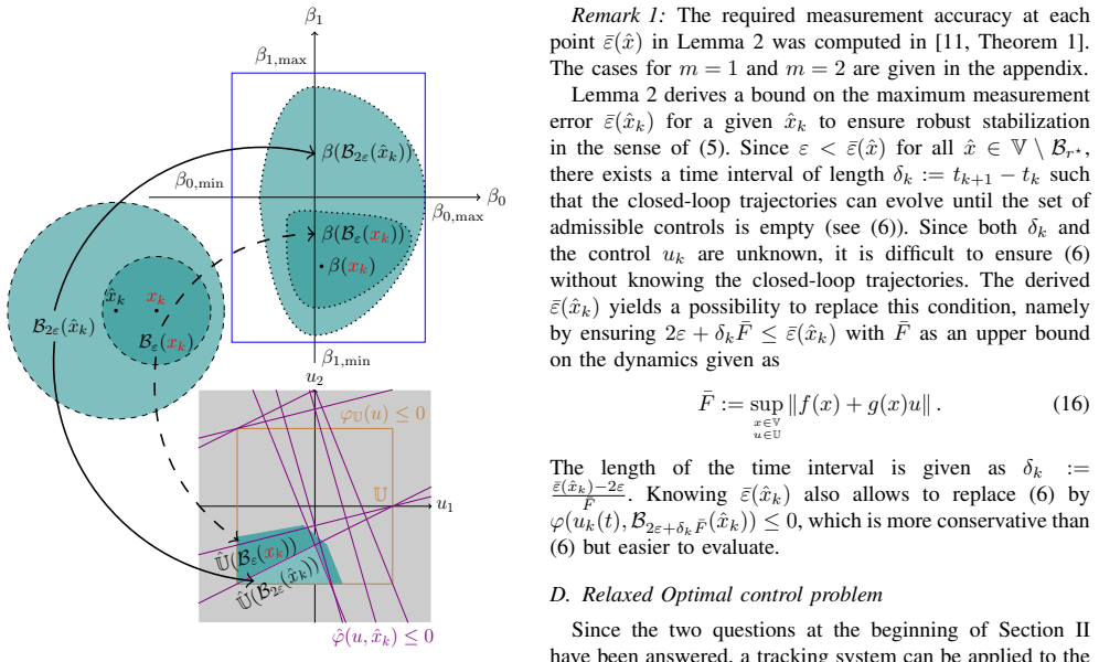
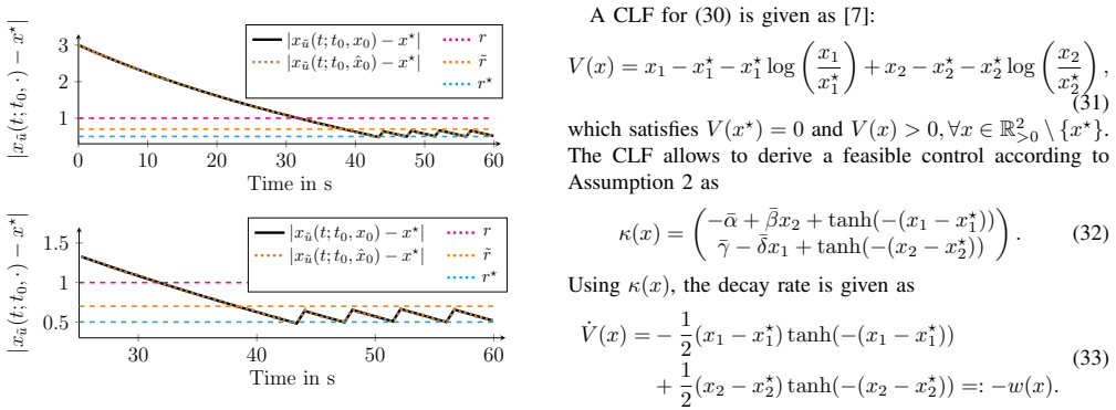
Solving optimal control problems to determine a stabilizing controller involves a significant computational effort. Time-varying optimal control provides a remedy by designing a tracking system, given as an ordinary differential equation, to track the solution of the optimal control problem. To improve the applicability of the method, measurement errors are considered in this paper and it is described how these errors influence a control Lyapunov function-based decay condition. As a result of these investigations, input-affine constraints that meet the standard formulation and that describe the set of admissible controls are obtained. The paper also derives a requirement on the necessary measurement accuracy as well as a triggering condition for taking a new measurement. The main theorem combines these results into a robustly stabilizing control algorithm, meaning that all closed-loop trajectories starting in a vicinity around the true state converge to zero. Additionally, the tracking system ensures that the optimal control is tracked at the end of each sampling period. The effectiveness of this approach is demonstrated using a train acceleration model and the well-known predator-prey model.
Editorial analysis
A structured set of objections, weighed in public.
Referee Report
Summary. The manuscript proposes an approach to time-varying optimal control that incorporates measurement errors. It examines the impact of these errors on a control Lyapunov function-based decay condition, resulting in input-affine admissible control sets, a measurement accuracy requirement, and a triggering condition. The central result is a main theorem that combines these elements into a robustly stabilizing algorithm, ensuring that closed-loop trajectories starting near the true state converge to zero, while the tracking system follows the optimal control at sampling instants. The method is validated on a train acceleration model and the predator-prey model.
Significance. Should the main stability theorem hold, the paper offers a valuable contribution by extending time-varying optimal control techniques to account for realistic measurement imperfections. This could enhance the applicability of such methods in practical control systems where sensor noise is inevitable. The derivation of triggering conditions to balance measurement accuracy and stability is particularly promising for resource-constrained applications.
major comments (1)
- [Main Theorem and stability analysis] Main Theorem (as described in the abstract): The assertion that closed-loop trajectories converge to zero under bounded measurement errors is load-bearing for the central claim but requires verification. The CLF decay condition is perturbed by a term proportional to the measurement error. Without an explicit ISS-gain argument or demonstration that the integrated perturbation vanishes (e.g., via the triggering condition forcing error to zero asymptotically), trajectories may converge only to a neighborhood whose radius depends on the error bound, yielding practical stability rather than asymptotic stability to the origin. The derivation of the admissible control sets and triggering condition should include a concrete proof step addressing this.
minor comments (2)
- [Abstract] The abstract refers to 'input-affine constraints that meet the standard formulation' without specifying the underlying system class (e.g., control-affine nonlinear dynamics). Adding this detail would improve precision.
- [Demonstration section] In the numerical examples, include quantitative data on triggering frequency and the size of the ultimate bound under different error levels to better illustrate the practical implications of the accuracy requirement.
Simulated Author's Rebuttal
We thank the referee for the careful reading of our manuscript and the constructive comments. We provide a point-by-point response to the major comment below.
read point-by-point responses
-
Referee: The assertion that closed-loop trajectories converge to zero under bounded measurement errors is load-bearing for the central claim but requires verification. The CLF decay condition is perturbed by a term proportional to the measurement error. Without an explicit ISS-gain argument or demonstration that the integrated perturbation vanishes (e.g., via the triggering condition forcing error to zero asymptotically), trajectories may converge only to a neighborhood whose radius depends on the error bound, yielding practical stability rather than asymptotic stability to the origin. The derivation of the admissible control sets and triggering condition should include a concrete proof step addressing this.
Authors: We agree that the stability analysis requires careful verification to confirm asymptotic rather than practical stability. In the manuscript, the triggering condition is formulated to ensure that the measurement error remains sufficiently small relative to the current state norm at all times, specifically by enforcing that the perturbation term in the CLF derivative is dominated by the negative definite term. This is achieved without requiring the error to vanish asymptotically; instead, the admissible control set is chosen input-affine to compensate for the bounded error. The proof of the main theorem uses a direct comparison with a nominal decay rate and shows that the state cannot remain away from zero. However, to address the referee's concern, we will add an explicit lemma showing that the integrated effect of the perturbation is controlled by the trigger, leading to lim |x(t)| = 0 as t to infinity. This will be included in the revised manuscript. revision: yes
Circularity Check
No circularity: derivation proceeds from standard CLF decay under explicit perturbation
full rationale
The paper starts from the standard control-Lyapunov-function decay inequality, inserts a measurement-error term that is treated as an exogenous bounded perturbation, and algebraically derives the resulting input-affine admissible set, accuracy threshold, and triggering rule. These steps are forward derivations, not redefinitions or fits of the target stability statement. The main theorem simply assembles the three derived objects; no equation is shown to be identical to its own input by construction, and no load-bearing uniqueness claim rests on a self-citation. The abstract and reader summary confirm reliance on external CLF literature rather than internal re-use of the paper’s own fitted quantities.
Axiom & Free-Parameter Ledger
axioms (2)
- standard math Existence and uniqueness of solutions for the ordinary differential equations describing the tracking system and closed-loop dynamics.
- domain assumption The control Lyapunov function decay condition can be adjusted for bounded measurement errors while preserving input-affine structure.
Reference graph
Works this paper leans on
- [1]
-
[2]
M. Fazlyab, C. Nowzari, G. J. Pappas, A. Ribeiro, and V . M. Preciado. Self-triggered time-varying convex optimization. InProc. of the 55th IEEE Conference on Decision and Control (CDC), pages 3090–3097. IEEE, 2016
work page 2016
-
[3]
M. Fazlyab, S. Paternain, V . M. Preciado, and A. Ribeiro. Prediction- correction interior-point method for time-varying convex optimization. IEEE Transactions on Automatic Control (TAC), 63(7):1973–1986, 2017
work page 1973
-
[4]
L. Gr ¨une and J. Pannek. Nonlinear Model Predictive Control. In Nonlinear Model Predictive Control, pages 45–69. Springer, 2017
work page 2017
- [5]
-
[6]
H. Khalil.Nonlinear Systems. Prentice-Hall. 3rd edition, 2002
work page 2002
-
[7]
M. E. M. Meza, A. Bhaya, and E. Kaszkurewicz. Controller design techniques for the Lotka-Volterra nonlinear system.Sba: Controle & Automac ¸˜ao Sociedade Brasileira de Automatica, 16:124–135, 2005
work page 2005
- [8]
-
[9]
P. Schmidt, T. G ¨ohrt, and S. Streif. Tracking of stabilizing, optimal control in fixed-time based on time-varying objective function.Proc. of the 60th IEEE Conference on Decision and Control (CDC), pages 6012–6017, 2021
work page 2021
-
[10]
P. Schmidt, P. Osinenko, and S. Streif. On inf-convolution-based robust practical stabilization under computational uncertainty.IEEE Transactions on Automatic Control (TAC), 66(11):5530–5537, 2021
work page 2021
-
[11]
P. Schmidt, P. Osinenko, and S. Streif. Some remarks on practical stabilization via CLF-based control under measurement noise.IEEE Access, 13:1882–1895, 2024
work page 2024
-
[12]
A. Simonetto, E. Dall’Anese, S. Paternain, G. Leus, and G. B. Gian- nakis. Time-varying convex optimization: Time-structured algorithms and applications.Proceedings of the IEEE, 108(11):2032–2048, 2020
work page 2032
-
[13]
A. Simonetto, A. Mokhtari, A. Koppel, G. Leus, and A. Ribeiro. A class of prediction-correction methods for time-varying convex optimization.IEEE Transactions on Signal Processing (TSP), 64(17):4576–4591, 2016
work page 2016
-
[14]
E. D. Sontag. Stability and stabilization: discontinuities and the effect of disturbances. InNonlinear Analysis, Differential Equations and Control, pages 551–598. Springer, 1999. APPENDIX The required measurement accuracy (see Lemma 2) was computed in [11] and is given as ¯ε(x) = ¯ε0,ifβ 0(x)≤0∧β 1(x) = 0 ¯ε1,ifβ 0(x)>0∧β 1(x)̸= 0 min{¯ε0,¯ε1},el...
work page 1999
discussion (0)
Sign in with ORCID, Apple, or X to comment. Anyone can read and Pith papers without signing in.