Quantum Data Loading for Carleman Linearized Systems: Application to the Lattice-Boltzmann Equation
Pith reviewed 2026-05-21 00:27 UTC · model grok-4.3
The pith
A matrix decomposition turns arbitrary operators into linear combinations of unitaries whose term count stays independent of grid size for Carleman-linearized systems like the lattice Boltzmann equation.
A machine-rendered reading of the paper's core claim, the machinery that carries it, and where it could break.
Core claim
The authors introduce a decomposition that converts an arbitrary square matrix into a linear combination of non-unitaries and then embeds each non-unitary term inside a unitary, yielding a linear combination of unitaries with an equal number of terms. They show that this decomposition produces a generalized linear combination of unitaries framework for any Carleman-linearized autonomous dynamical system possessing a polynomial nonlinearity. For the three-dimensional Carleman-linearized lattice Boltzmann equation the number of terms scales as O(alpha squared Q squared), where alpha is the truncation order and Q is the number of discrete velocities, and this count is completely independent of
What carries the argument
The decomposition of an arbitrary square matrix into a linear combination of non-unitaries that each embed into unitaries to form a linear combination of unitaries with the same term count.
If this is right
- The linear combination of unitaries for the three-dimensional Carleman-linearized lattice Boltzmann equation has a term count that scales as O(alpha squared Q squared).
- The term count remains independent of both the number of temporal and spatial discretization points.
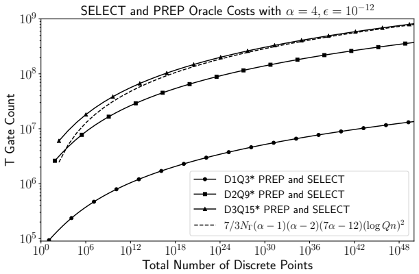
- Combined with preparation and selection oracles the T-gate cost scales as O(alpha cubed Q squared times the square of the log of the number of grid points).
- When paired with the variational quantum linear solver the approach requires a number of circuits per iteration equal to the square of the term count times a logarithmic factor involving time steps and the Carleman order.
Where Pith is reading between the lines
- The same decomposition approach could be applied to other nonlinear partial differential equations that admit Carleman linearization, such as reaction-diffusion or Navier-Stokes systems.
- If the term count truly stays independent of grid size, quantum resource estimates for fluid simulations would improve markedly when moving to finer meshes.
- Small-scale numerical tests of the decomposition on toy matrices drawn from the lattice Boltzmann system could directly verify the claimed independence from discretization.
Load-bearing premise
An arbitrary square matrix can be decomposed into a linear combination of non-unitaries with a term count that does not grow with the number of spatial grid points or time steps.
What would settle it
Apply the decomposition to the system matrix for two different spatial grid resolutions and check whether the number of terms in the resulting linear combination of unitaries remains unchanged.
Figures



read the original abstract
Herein, we introduce a strategy to decompose an arbitrary square matrix into a linear combination of non-unitaries (LCNU) where each non-unitary term is embedded into a unitary matrix. The result is a linear combination of unitaries (LCU) with an equal number of terms as the LCNU. Using this approach, we construct a generalized LCU framework for any Carleman linearized autonomous dynamical system with a polynomial nonlinearity. This framework is then used to construct an LCU for the 3-dimensional Carleman linearized lattice Boltzmann equation (LBE) in which the number of terms scales like $N_s \sim \mathcal{O}(\alpha^2 Q^2)$, where $\alpha$ is the Carleman truncation order and $Q$ is the number of discrete velocities from the LBE. Importantly, $N_s$ is completely independent of both the number of temporal and spatial discretization points. Lastly, we provide an estimate of our LCNU strategy's T gate cost in conjunction with (1) PREP and SELECT block encoding oracles, and (2) the variational quantum linear solver. In the former, the T cost scales like $\mathcal{O}(\alpha^3 Q^2 (\log_2 n)^2)$, where $n$ is the total number of spatial grid points across all dimensions. Next, the latter requires $N_s^2(\log_2 (2n_tn^\alpha)+1)$ circuits per iteration, with a worst case T gate cost of $\mathcal{O}(\alpha (\log_2 Qn)^2)$ among them. We, therefore, provide an efficient decomposition strategy useful for both fault-tolerant and variational approaches.
Editorial analysis
A structured set of objections, weighed in public.
Referee Report
Summary. The paper introduces a strategy to decompose an arbitrary square matrix into a linear combination of non-unitaries (LCNU), each embeddable in a unitary, yielding an LCU with equal term count. This is generalized to any Carleman-linearized autonomous dynamical system with polynomial nonlinearity and applied to construct an LCU for the 3D Carleman-linearized lattice Boltzmann equation (LBE), with term count Ns scaling as O(α² Q²) independent of spatial grid points n and time steps nt. T-gate cost estimates are given for PREP/SELECT block encodings and the variational quantum linear solver.
Significance. If the central decomposition holds with the claimed scaling, the work would provide a route to quantum simulation of fluid dynamics via LBE that avoids exponential growth in operator terms with discretization size, a potentially important step toward practical quantum advantage in computational fluid dynamics. The explicit T-cost scaling for both fault-tolerant and variational settings adds concrete utility if the underlying LCNU construction is rigorous.
major comments (2)
- [Abstract] Abstract (paragraph beginning 'Herein, we introduce a strategy...'): The general LCNU decomposition for an arbitrary square matrix is presented as achieving term count equal to the final LCU without additional dimension-dependent factors. For the Carleman-linearized LBE the operator dimension scales as n^α; a generic decomposition into non-unitaries would normally produce term count growing with this dimension unless the construction explicitly cancels the n dependence via the tensor-product structure of the LBE streaming and collision operators. The manuscript must supply the explicit construction and proof that this cancellation occurs for arbitrary matrices before the independence claim can be accepted.
- [LBE application section] Section on application to 3D LBE (following the generalized framework): The reported Ns ∼ O(α² Q²) independent of n and nt is load-bearing for the headline result. Without a concrete decomposition of the Carleman-expanded LBE operator that demonstrates how the general LCNU avoids introducing factors proportional to n^α or nt, the scaling cannot be verified and may rest on an unstated structural cancellation specific to LBE rather than the claimed generality.
minor comments (2)
- [T-gate cost estimates] The T-gate cost expressions (O(α³ Q² (log₂ n)²) for PREP/SELECT and O(α (log₂ Q n)²) worst-case for VQLS) would benefit from an explicit breakdown of the PREP and SELECT oracle implementations and how the LCNU terms enter the circuit depth.
- Notation for the Carleman truncation order α and discrete velocity count Q should be defined at first use with a brief reminder of their relation to the underlying LBE discretization.
Simulated Author's Rebuttal
We thank the referee for their detailed and constructive comments. We address each of the major comments below and indicate the revisions we will make to the manuscript.
read point-by-point responses
-
Referee: The general LCNU decomposition for an arbitrary square matrix is presented as achieving term count equal to the final LCU without additional dimension-dependent factors. For the Carleman-linearized LBE the operator dimension scales as n^α; a generic decomposition into non-unitaries would normally produce term count growing with this dimension unless the construction explicitly cancels the n dependence via the tensor-product structure of the LBE streaming and collision operators. The manuscript must supply the explicit construction and proof that this cancellation occurs for arbitrary matrices before the independence claim can be accepted.
Authors: We agree that an explicit construction is essential to substantiate the scaling claim. Our LCNU approach begins with a decomposition of the original system operators, which for the LBE are highly structured (local collision and streaming terms with tensor-product form across grid points). The Carleman linearization preserves this structure in a block-wise manner, allowing the LCNU to be applied to the base operators and extended via Kronecker products without introducing additional factors of n or nt. The generalized framework in Section 2 details this for any polynomial system, and Section 3 applies it to LBE showing the O(α² Q²) scaling. To address the concern, we will add an appendix with the full proof of the term count independence, including the explicit LCNU terms for the LBE operator. revision: yes
-
Referee: The reported Ns ∼ O(α² Q²) independent of n and nt is load-bearing for the headline result. Without a concrete decomposition of the Carleman-expanded LBE operator that demonstrates how the general LCNU avoids introducing factors proportional to n^α or nt, the scaling cannot be verified and may rest on an unstated structural cancellation specific to LBE rather than the claimed generality.
Authors: The concrete decomposition is provided in the LBE application section, where we expand the Carleman-linearized operator and identify the distinct non-unitary components arising from the velocity discretizations and polynomial terms up to order α. Because the spatial grid enters only through identical local operators tensored across sites, the number of unique terms does not grow with n. Similarly, the time discretization does not affect the operator itself in the linear system formulation. We acknowledge that the presentation could be more explicit, and we will revise the section to include a table or diagram listing the LCNU terms and their embeddings, thereby verifying the claimed scaling directly from the construction rather than relying on the general framework alone. revision: yes
Circularity Check
No circularity: derivation presents explicit algorithmic construction independent of target scaling.
full rationale
The paper introduces a decomposition strategy for arbitrary square matrices into LCNU (with equal-term LCU embedding) as a new contribution, then applies the resulting generalized LCU framework to Carleman-linearized polynomial systems and specifically to the 3D LBE operator. The claimed Ns ~ O(α² Q²) scaling independent of n and nt is stated as following directly from the operator structure under this framework. No equation or section reduces a prediction to a fitted parameter, self-citation chain, or definitional renaming; the central result is an explicit construction rather than a re-expression of inputs. This is the normal case of a self-contained algorithmic paper.
Axiom & Free-Parameter Ledger
axioms (2)
- domain assumption Carleman linearization of a polynomial nonlinearity yields a finite-dimensional linear system after truncation at order α
- ad hoc to paper Any square matrix admits a decomposition into a linear combination of non-unitaries that can each be embedded in a unitary with equal term count
Lean theorems connected to this paper
-
IndisputableMonolith/Foundation/AbsoluteFloorClosure.leanreality_from_one_distinction unclear?
unclearRelation between the paper passage and the cited Recognition theorem.
We construct a generalized LCU framework for any Carleman linearized autonomous dynamical system with a polynomial nonlinearity... Ns ∼ O(α² Q²) ... completely independent of both the number of temporal and spatial discretization points.
-
IndisputableMonolith/Cost/FunctionalEquation.leanwashburn_uniqueness_aczel unclear?
unclearRelation between the paper passage and the cited Recognition theorem.
Decomposition of the F1 Matrix ... Decomposition of the F2 and F3 Matrices ... Explicit Circuit Constructions
What do these tags mean?
- matches
- The paper's claim is directly supported by a theorem in the formal canon.
- supports
- The theorem supports part of the paper's argument, but the paper may add assumptions or extra steps.
- extends
- The paper goes beyond the formal theorem; the theorem is a base layer rather than the whole result.
- uses
- The paper appears to rely on the theorem as machinery.
- contradicts
- The paper's claim conflicts with a theorem or certificate in the canon.
- unclear
- Pith found a possible connection, but the passage is too broad, indirect, or ambiguous to say the theorem truly supports the claim.
Reference graph
Works this paper leans on
-
[1]
Define the set of tuples Λ1 := {(i, j, l, η, p, m) |i ∈ {1, 2}, j ∈ {1,
Circuits for L(e) lin,1: Streaming Term We now turn our attention to the streaming terms associated with S. Define the set of tuples Λ1 := {(i, j, l, η, p, m) |i ∈ {1, 2}, j ∈ {1, . . . α}, l ∈ {0, . . . , j − 1}, η ∈ {x, y, z}, p ∈ {+1, −1}, m ∈ {1, . . . , NEη }}. Then, by combining (25) with the linear component of (26) and inserting (15) and (53), we ...
-
[2]
Define the set of tuples Λ2 = {(i, j, l, m) | i ∈ {1, 2}, j ∈ {1,
Circuits for L(e) lin,2: Linear Collision Term We now turn our attention to the linear collision terms associated with ˜F1. Define the set of tuples Λ2 = {(i, j, l, m) | i ∈ {1, 2}, j ∈ {1, . . . α}, l ∈ {0, . . . , j − 1}, m ∈ {1, . . . , NR}}. Then, by combining (25) with the linear component of (26) and inserting (15) and (43), we obtain L(e) lin,2 = X...
-
[3]
First, define the set of tuples Λ3 = {(k, i, j, l, q, m) |k ∈ {2, 3}, i ∈ {1, 2}, j ∈ {1,
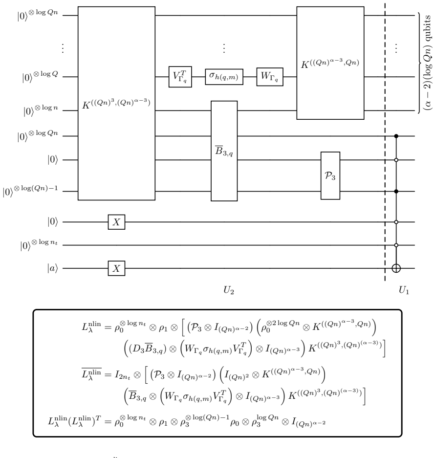
Circuits for L(e) nlin: Nonlinear Collision Terms The final component to analyze is L(e) nlin, which contains both the quadratic and cubic nonlinear collision terms. First, define the set of tuples Λ3 = {(k, i, j, l, q, m) |k ∈ {2, 3}, i ∈ {1, 2}, j ∈ {1, . . . , α− k + 1}, l ∈ {0, . . . , j − 1}, q ∈ {1, . . . , Q}, m ∈ {1, . . . , NΓq }}. 23 ... ... |0⟩...
-
[4]
T Count for L(e) 1 Terms By applying (74) to the controlled L1,i terms of (76), we have G[CU(L1,i)] = G[CL1,i] + G[C T (L1,i)+1X] for i = 1, 2, 3. From the completions in (63) and using rows 1 and 5 from Table II, we find 3X i=1 G[CL1,i] = log ntG[CX ] + G[CS nt +1] = 12 log 2nt. (77) Next, with (64) we find that T (L1,1) = 0, T (L1,2) = log nt, and T (L1...
-
[5]
From (66), we see that G[CLlin,1 λ ] = G[CS η,p,m]
T Count for L(e) lin,1 Terms Next, from (65b) and (74), we see that G[CU(Llin,1 λ )] = G[CLlin,1 λ ] + G[C T (Llin,1 λ )+1X] for a given λ ∈ Λ1. From (66), we see that G[CLlin,1 λ ] = G[CS η,p,m]. Using the definition of Sη,p,m from (54) and assuming NEx = NEy = NEz, we find X λ∈Λ1 G[CLlin,1 λ ] = X λ∈Λ1 G[CS η,p,m] = α(α + 1)NEx X p∈{+1,−1} G[CS nx p ] +...
-
[6]
T Count for L(e) lin,2 Terms Next, using (74) with the Llin,2 λ terms (68b) for λ ∈ Λ2, we have G[CU(Llin,2 λ )] = G[CLlin,2 λ ] + G[C T (Llin,2 λ )+1X]. From the completion in (69), and given that the T cost for any controlled Pauli gate is zero, we find that X λ∈Λ2 G[CLlin,2 λ ] = NRα(α + 1)(G[CW R] + G[CV R]), (83) where G[CW R] and G[CV R] are found n...
-
[7]
We make the assumption that G[CWΓq] = G[CWΓ] and G[CVΓq] = G[CVΓ] for all q ∈ { 1,
T Count for L(e) nlin Terms Next, using (74) with theLnlin λ terms (71b) for λ ∈ Λ3, we haveG[CU(Lnlin λ )] = G[CLnlin λ ]+G[C T (Lnlin λ )+1X]. We make the assumption that G[CWΓq] = G[CWΓ] and G[CVΓq] = G[CVΓ] for all q ∈ { 1, . . . , Q}, where G[CWΓ] = max{G[CWΓq] | q ∈ {1, . . . , Q}} and G[CVΓ] = max{G[CVΓq] | q ∈ {1, . . . , Q}}. Then, from the compl...
-
[8]
J.-P. Liu, H. Ø. Kolden, H. K. Krovi, N. F. Loureiro, K. Trivisa, and A. M. Childs, Efficient quantum algorithm for dissipative nonlinear differential equations, Proceedings of the National Academy of Sciences 118, e2026805118 (2021)
work page 2021
-
[9]
K. Kowalski and W.-h. Steeb, Nonlinear dynamical systems and Carleman linearization (World Scientific, 1991)
work page 1991
-
[10]
A. M. Childs, R. Kothari, and R. D. Somma, Quantum algorithm for systems of linear equations with exponen- tially improved dependence on precision, SIAM Journal on Computing 46, 1920–1950 (2017)
work page 1920
-
[11]
A. W. Harrow, A. Hassidim, and S. Lloyd, Quantum algorithm for linear systems of equations, Physical Review Letters 103, 10.1103/physrevlett.103.150502 (2009)
-
[12]
C. Bravo-Prieto, R. LaRose, M. Cerezo, Y. Subasi, L. Cincio, and P. J. Coles, Variational quantum linear solver, Quantum 7, 1188 (2023)
work page 2023
- [13]
-
[14]
A. M. Dalzell, A shortcut to an optimal quantum linear system solver, arXiv preprint arXiv:2406.12086 (2024)
work page internal anchor Pith review Pith/arXiv arXiv 2024
-
[15]
Aaronson, Read the fine print, Nature Physics 11, 291 (2015)
S. Aaronson, Read the fine print, Nature Physics 11, 291 (2015)
work page 2015
-
[16]
L. Hantzko, L. Binkowski, and S. Gupta, Tensorized pauli decomposition algorithm, Physica Scripta 99, 085128 (2024)
work page 2024
-
[17]
A. Gnanasekaran and A. Surana, Efficient variational quantum linear solver for structured sparse matrices, in 2024 IEEE International Conference on Quantum Computing and Engineering (QCE) (IEEE, 2024) p. 199–210
work page 2024
-
[18]
A. Gnanasekaran and A. Surana, Efficient quantum access model for sparse structured matrices using linear combination of “things”, Physical Review A 113, 022437 (2026)
work page 2026
-
[19]
A. Surana and A. Gnanasekaran, Variational quantum framework for partial differential equation constrained optimization, ACM Transactions on Quantum Computing 7, 1 (2025)
work page 2025
- [20]
-
[21]
J. Bae, G. Yoo, S. Nakamura, S. Ohnishi, and D. S. Kim, Hardware efficient decomposition of the laplace operator and its application to the helmholtz and the poisson equation on quantum computer, Quantum Information Processing 23, 10.1007/s11128-024-04458-y (2024)
- [22]
- [23]
-
[24]
R. Demirdjian, T. Hogancamp, and D. Gunlycke, Efficient decomposition of the carleman linearized burgers’ equation, Phys. Rev. A 10.1103/g27q-r2gk (2026). 35
-
[25]
R. Demirdjian, D. Gunlycke, C. A. Reynolds, J. D. Doyle, and S. Tafur, Variational quantum solutions to the advection–diffusion equation for applications in fluid dynamics, Quantum Information Processing 21, 10.1007/s11128-022-03667-7 (2022)
- [26]
-
[27]
T. Nguyen, Quantum algorithms for partial differential equations: A performance review and future trajectories, in Intelligent Sustainable Systems , edited by N. Atulya K., J. Dharm Singh, M. Durgesh Kumar, and A. Joshi (Springer Nature Switzerland, Cham, 2025) pp. 18–37
work page 2025
-
[28]
S. S. Bharadwaj and K. R. Sreenivasan, Compact quantum algorithms for time-dependent differential equations, Physical Review Research 7, 023262 (2025)
work page 2025
-
[29]
D. Jennings, K. Korzekwa, M. Lostaglio, P. Mannix, R. Ashworth, E. Marsili, and S. Rolston, Simulating non- trivial incompressible flows with a quantum lattice boltzmann algorithm, inAIAA SCITECH 2026 Forum (2026) p. 1936
work page 2026
- [30]
- [32]
-
[33]
Z. Song, R. Deaton, B. Gard, and S. H. Bryngelson, Incompressible navier–stokes solve on noisy quantum hardware via a hybrid quantum–classical scheme, Computers & Fluids 288, 106507 (2025)
work page 2025
-
[34]
H.-C. Wu, J. Wang, and X. Li, Quantum algorithms for nonlinear dynamics: Revisiting carleman linearization with no dissipative conditions, SIAM Journal on Scientific Computing 47, A943 (2025)
work page 2025
-
[35]
A. Surana, A. Gnanasekaran, and T. Sahai, An efficient quantum algorithm for simulating polynomial dynamical systems, Quantum Information Processing 23, 10.1007/s11128-024-04311-2 (2024)
-
[36]
N. Gourianov, P. Givi, D. Jaksch, and S. B. Pope, Tensor networks enable the calculation of turbulence probability distributions, Science Advances 11, eads5990 (2025), https://www.science.org/doi/pdf/10.1126/sciadv.ads5990
-
[37]
M. C. Garrett, D. Ponkratov, and W. Qiu, Feasibility of accelerating incompressible computational fluid dynamics simulations with fault-tolerant quantum computers, Marine Technology Society Journal 59, 62 (2025)
work page 2025
-
[38]
D. Jennings, M. Lostaglio, R. B. Lowrie, S. Pallister, and A. T. Sornborger, The cost of solving linear differential equations on a quantum computer: fast-forwarding to explicit resource counts, Quantum 8, 1553 (2024)
work page 2024
-
[39]
F. Tennie and T. N. Palmer, Quantum computers for weather and climate prediction: The good, the bad, and the noisy, Bulletin of the American Meteorological Society 104, E488–E500 (2023)
work page 2023
-
[40]
Finding flows of a Navier–Stokes fluid through quantum computing,
F. Gaitan, Finding flows of a navier–stokes fluid through quantum computing, npj Quantum Information 6, 10.1038/s41534-020-00291-0 (2020)
-
[41]
C. A. Williams, A. A. Gentile, V. E. Elfving, D. Berger, and O. Kyriienko, Quantum iterative methods for solving differential equations with application to computational fluid dynamics, Advanced Quantum Technologies , e00618 (2025)
work page 2025
-
[42]
F. Oz, R. K. S. S. Vuppala, K. Kara, and F. Gaitan, Solving burgers’ equation with quantum computing, Quantum Information Processing 21, 10.1007/s11128-021-03391-8 (2021)
- [43]
-
[44]
L. Lapworth, A hybrid quantum-classical cfd methodology with benchmark hhl solutions, arXiv preprint arXiv:2206.00419 (2022)
-
[45]
B. Ljubomir, Quantum algorithm for the navier–stokes equations by using the streamfunction-vorticity formulation and the lattice boltzmann method, International Journal of Quantum Information 20, 10.1142/s0219749921500398 (2022)
-
[46]
M. Lubasch, J. Joo, P. Moinier, M. Kiffner, and D. Jaksch, Variational quantum algorithms for nonlinear prob- lems, Physical Review A 101, 10.1103/physreva.101.010301 (2020)
-
[47]
T. Hogancamp, R. Demirdjian, and D. Gunlycke, A linear combination of unitaries decomposition for the laplace operator, arXiv preprint arXiv:2601.06370 (2026)
-
[48]
Y. Gan, H. Alipanah, J. Cheng, Z. Wu, G. Li, J. J. Mendoza-Arenas, P. Givi, M. R. Malik, B. J. McDermott, and J. Liu, Provably efficient quantum algorithms for solving nonlinear differential equations using multiple bosonic 36 modes coupled with qubits, arXiv preprint arXiv:2511.09939 (2025)
-
[49]
J. Gonzalez-Conde, D. Lewis, S. S. Bharadwaj, and M. Sanz, Quantum carleman linearization efficiency in nonlinear fluid dynamics, Physical Review Research 7, 023254 (2025)
work page 2025
- [50]
-
[51]
D. Jennings, K. Korzekwa, M. Lostaglio, A. T. Sornborger, Y. Subasi, and G. Wang, Quantum algorithms for general nonlinear dynamics based on the carleman embedding, arXiv preprint arXiv:2509.07155 (2025)
-
[53]
W. Itani and S. Succi, Analysis of carleman linearization of lattice boltzmann, Fluids 7, 24 (2022)
work page 2022
-
[54]
C. Sanavio and S. Succi, Lattice boltzmann–carleman quantum algorithm and circuit for fluid flows at moderate reynolds number, AVS Quantum Science 6 (2024)
work page 2024
-
[55]
C. Sanavio, R. Scatamacchia, C. De Falco, and S. Succi, Three carleman routes to the quantum simulation of classical fluids, Physics of Fluids 36 (2024)
work page 2024
- [56]
-
[57]
C. Sanavio, W. A. Simon, A. Ralli, P. Love, and S. Succi, Carleman-lattice-boltzmann quantum circuit with matrix access oracles, Physics of Fluids 37 (2025)
work page 2025
-
[58]
D. Jennings, K. Korzekwa, M. Lostaglio, R. Ashworth, E. Marsili, and S. Rolston, An end-to-end quantum algo- rithm for nonlinear fluid dynamics with bounded quantum advantage, arXiv preprint arXiv:2512.03758 (2025)
-
[59]
B. Kramer and G. Pogudin, Discovering polynomial and quadratic structure in nonlinear ordinary differential equations, arXiv preprint arXiv:2502.10005 (2025)
-
[60]
C. Xu, L. He, and Z. Lin, Commutation matrices and commutation tensors, Linear and Multilinear Algebra 68, 1721 (2018)
work page 2018
-
[61]
T. Kr¨ uger, H. Kusumaatmaja, A. Kuzmin, O. Shardt, G. Silva, and E. M. Viggen,The lattice Boltzmann method , Vol. 10 (Springer, 2017)
work page 2017
-
[62]
P. L. Bhatnagar, E. P. Gross, and M. Krook, A model for collision processes in gases. i. small amplitude processes in charged and neutral one-component systems, Phys. Rev. 94, 511 (1954)
work page 1954
-
[63]
X. Li, X. Yin, N. Wiebe, J. Chun, G. K. Schenter, M. S. Cheung, and J. M¨ ulmenst¨ adt, Potential quantum advantage for simulation of fluid dynamics, Physical Review Research 7, 013036 (2025)
work page 2025
-
[64]
Tutorial on the Quantikz Package
A. Kay, Tutorial on the quantikz package, arXiv preprint arXiv:1809.03842 (2018)
-
[65]
A. M. Childs and N. Wiebe, Hamiltonian simulation using linear combinations of unitary operations, arXiv preprint arXiv:1202.5822 (2012)
work page internal anchor Pith review Pith/arXiv arXiv 2012
-
[66]
S. Hariprakash, N. S. Modi, M. Kreshchuk, C. F. Kane, and C. W. Bauer, Strategies for simulating the time evolution of hamiltonian lattice field theories, Physical Review A 111, 022419 (2025)
work page 2025
-
[67]
Selinger, Quantum circuits of t-depth one, Phys
P. Selinger, Quantum circuits of t-depth one, Phys. Rev. A 87, 042302 (2013)
work page 2013
-
[68]
T. Khattar and C. Gidney, Rise of conditionally clean ancillae for efficient quantum circuit constructions, Quan- tum 9, 1752 (2025)
work page 2025
-
[69]
Constructing large increment gates (2015)
work page 2015
-
[70]
P. MQ Cruz and B. Murta, Shallow unitary decompositions of quantum fredkin and toffoli gates for connectivity- aware equivalent circuit averaging, APL Quantum 1 (2024)
work page 2024
-
[71]
A. Gnanasekaran, A. Surana, and H. Zhu, Variational quantum framework for nonlinear pde constrained opti- mization using carleman linearization, Quantum Information & Computation 25, 260 (2025)
work page 2025
-
[72]
A. Javadi-Abhari, M. Treinish, K. Krsulich, C. J. Wood, J. Lishman, J. Gacon, S. Martiel, P. D. Nation, L. S. Bishop, A. W. Cross, et al. , Quantum computing with qiskit, arXiv preprint arXiv:2405.08810 (2024)
work page internal anchor Pith review Pith/arXiv arXiv 2024
-
[73]
L. Lapworth and C. S¨ underhauf, Preconditioned block encodings for quantum linear systems, Quantum Science and Technology 10, 045064 (2025)
work page 2025
- [74]
- [75]
- [76]
-
[77]
M. Larocca, S. Thanasilp, S. Wang, K. Sharma, J. Biamonte, P. J. Coles, L. Cincio, J. R. McClean, Z. Holmes, and M. Cerezo, Barren plateaus in variational quantum computing, Nature Reviews Physics , 1 (2025)
work page 2025
-
[78]
A. J. Pool, A. D. Somoza, C. Mc Keever, M. Lubasch, and B. Horstmann, Nonlinear dynamics as a ground-state solution on quantum computers, Physical Review Research 6, 033257 (2024)
work page 2024
-
[79]
C. M. Keller, S. Eidenbenz, A. B¨ artschi, D. O’Malley, J. Golden, and S. Misra, Hierarchical multigrid ansatz for variational quantum algorithms, in ISC High Performance 2024 Research Paper Proceedings (39th International Conference) (2024) pp. 1–11
work page 2024
-
[80]
Efficient algorithm for generating Pauli coordinates for an arbitrary linear operator,
D. Gunlycke, M. C. Palenik, A. R. Emmert, and S. A. Fischer, Efficient algorithm for generating pauli coordinates for an arbitrary linear operator, arXiv preprint arXiv:2011.08942 (2020)
-
[81]
T. Horstmann, Hybrid numerical methods based on the lattice Boltzmann approach with application to non- uniform grids , Ph.D. thesis, Universit´ e de Lyon (2018)
work page 2018
-
[82]
S¨ oderlind, The logarithmic norm
G. S¨ oderlind, The logarithmic norm. history and modern theory, BIT Numerical Mathematics 46, 631 (2006)
work page 2006
discussion (0)
Sign in with ORCID, Apple, or X to comment. Anyone can read and Pith papers without signing in.