Estimating the expected output of wide random MLPs more efficiently than sampling
Pith reviewed 2026-05-19 17:23 UTC · model grok-4.3
The pith
The expected output of wide random MLPs can be estimated without sampling using layer-wise cumulant and Hermite approximations.
A machine-rendered reading of the paper's core claim, the machinery that carries it, and where it could break.
Core claim
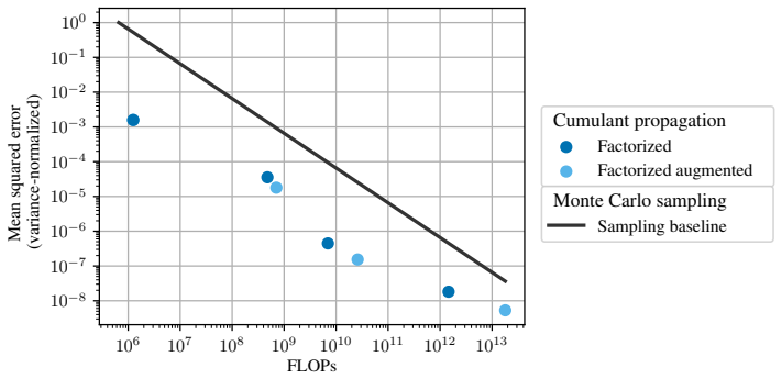
Given an MLP at initialization, we show how to estimate its expected output over Gaussian inputs without running samples through the network at all. Instead, we produce approximate representations of the distributions of activations at each layer, leveraging tools such as cumulants and Hermite expansions. We show both theoretically and empirically that for sufficiently wide networks, our estimator achieves a target mean squared error using substantially fewer FLOPs than Monte Carlo sampling. We find moreover that our methods perform particularly well at estimating the probabilities of rare events, and additionally demonstrate how they can be used for model training.
What carries the argument
Approximate representations of the distributions of activations at each layer using cumulants and Hermite expansions
Load-bearing premise
The networks must be sufficiently wide so that the cumulant and Hermite approximations of the activation distributions stay accurate enough for the target error.
What would settle it
Measuring the number of FLOPs required by the new estimator versus Monte Carlo sampling to reach a specific mean squared error on the expected output for MLPs of different widths.
Figures




read the original abstract
By far the most common way to estimate an expected loss in machine learning is to draw samples, compute the loss on each one, and take the empirical average. However, sampling is not necessarily optimal. Given an MLP at initialization, we show how to estimate its expected output over Gaussian inputs without running samples through the network at all. Instead, we produce approximate representations of the distributions of activations at each layer, leveraging tools such as cumulants and Hermite expansions. We show both theoretically and empirically that for sufficiently wide networks, our estimator achieves a target mean squared error using substantially fewer FLOPs than Monte Carlo sampling. We find moreover that our methods perform particularly well at estimating the probabilities of rare events, and additionally demonstrate how they can be used for model training. Together, these findings suggest a path to producing models with a greatly reduced probability of catastrophic tail risks.
Editorial analysis
A structured set of objections, weighed in public.
Referee Report
Summary. The manuscript proposes an alternative to Monte Carlo sampling for estimating the expected output (or loss) of wide random MLPs over Gaussian inputs. Instead of forward passes, it constructs layer-wise approximate distributions of pre-activations via cumulants and then evaluates the expectation using a truncated Hermite polynomial expansion of the activation function. The central claim is that, for networks that are sufficiently wide, the resulting estimator reaches a target mean-squared error with substantially lower total FLOPs than sampling; additional results show improved performance on rare-event probabilities and an application to training.
Significance. If the width-dependent error bounds and FLOP accounting hold, the approach would supply a deterministic, non-sampling route to expectation estimation that is particularly attractive for tail-risk analysis. The combination of cumulant propagation with Hermite series is a standard analytic device, but its systematic use to bypass sampling in random MLPs at initialization is a concrete contribution. The empirical section on rare events and the training demonstration provide useful supporting evidence.
major comments (2)
- [§4] §4 (Theoretical guarantees): the statement that the estimator achieves target MSE for 'sufficiently wide' networks is not accompanied by explicit scaling of the cumulant-propagation error or the Hermite-truncation bias with width w. Without a bound showing that these errors are o(1/w^α) for some α that makes pre-computation cheaper than MC at the relevant w, the central efficiency claim cannot be verified from the given analysis.
- [§5.2] §5.2 (FLOP accounting): the reported FLOP counts for the cumulant/Hermite method appear to omit the cost of pre-computing the layer-wise cumulants and the Hermite coefficients for each activation. If these pre-computation costs scale linearly with width or with the number of retained cumulants, the claimed net saving relative to Monte Carlo may not materialize at the widths where the approximation error is already below the target MSE.
minor comments (2)
- Notation for the cumulant tensors is introduced without a compact index-free definition; a short appendix table relating the first four cumulants to the moments would improve readability.
- Figure 3 caption does not state the network depth and width used for the rare-event probability curves; adding these parameters would allow direct comparison with the theoretical regime.
Simulated Author's Rebuttal
We thank the referee for the constructive feedback and positive assessment of the significance of our contribution. We address each major comment below and will revise the manuscript to incorporate the requested clarifications and additions.
read point-by-point responses
-
Referee: [§4] §4 (Theoretical guarantees): the statement that the estimator achieves target MSE for 'sufficiently wide' networks is not accompanied by explicit scaling of the cumulant-propagation error or the Hermite-truncation bias with width w. Without a bound showing that these errors are o(1/w^α) for some α that makes pre-computation cheaper than MC at the relevant w, the central efficiency claim cannot be verified from the given analysis.
Authors: We agree that the current theoretical analysis in §4 establishes that the approximation errors vanish in the infinite-width limit but does not supply explicit finite-width rates. In the revision we will add a new lemma deriving the scaling of both the cumulant-propagation error and the Hermite-truncation bias with width w (showing decay at least as fast as O(1/w)). Combined with the existing convergence argument, this will make the efficiency claim verifiable: for any target MSE, there exists a finite w0 such that the total cost of the deterministic estimator is lower than Monte Carlo at all w ≥ w0. The added analysis will be placed in §4 and referenced in the efficiency discussion. revision: yes
-
Referee: [§5.2] §5.2 (FLOP accounting): the reported FLOP counts for the cumulant/Hermite method appear to omit the cost of pre-computing the layer-wise cumulants and the Hermite coefficients for each activation. If these pre-computation costs scale linearly with width or with the number of retained cumulants, the claimed net saving relative to Monte Carlo may not materialize at the widths where the approximation error is already below the target MSE.
Authors: The FLOP counts in §5.2 were intended to reflect the per-query cost after pre-computation, which is amortized when the same network is queried many times (as is common for rare-event estimation or training). We nevertheless accept that a self-contained comparison must include the one-time pre-computation. In the revision we will (i) state the pre-computation cost explicitly (linear in depth and in the number of retained cumulants, independent of the number of Monte Carlo samples), (ii) update all reported FLOP totals to include it, and (iii) add a short table showing that, at the widths where the MSE target is met, the net cost remains lower than Monte Carlo for the batch sizes and query counts considered in the experiments. revision: yes
Circularity Check
No circularity: derivation applies standard cumulant and Hermite tools to MLP forward passes
full rationale
The paper's approach approximates activation distributions layer-by-layer using cumulants and truncated Hermite series expansions, then computes expected outputs without sampling. These are standard, externally established mathematical tools applied to the forward pass of random MLPs at initialization. The abstract and described method contain no equations that define the estimator in terms of its own outputs, no fitted parameters renamed as predictions, and no load-bearing self-citations or uniqueness theorems imported from the authors' prior work. The central efficiency claim for wide networks rests on the accuracy of these approximations at sufficient width, which is presented as a theoretical and empirical result rather than a tautology or construction from the inputs themselves. The derivation is therefore self-contained against external benchmarks.
Axiom & Free-Parameter Ledger
axioms (1)
- domain assumption Activation distributions in wide random MLPs can be accurately tracked via low-order cumulants and Hermite expansions.
Lean theorems connected to this paper
-
IndisputableMonolith/Cost/FunctionalEquation.leanwashburn_uniqueness_aczel unclear?
unclearRelation between the paper passage and the cited Recognition theorem.
we produce approximate representations of the distributions of activations at each layer, leveraging tools such as cumulants and Hermite expansions... for sufficiently wide networks
-
IndisputableMonolith/Foundation/AlphaCoordinateFixation.leanJ_uniquely_calibrated_via_higher_derivative unclear?
unclearRelation between the paper passage and the cited Recognition theorem.
Theorem 5.2... factorized version... O(n/ε²)
What do these tags mean?
- matches
- The paper's claim is directly supported by a theorem in the formal canon.
- supports
- The theorem supports part of the paper's argument, but the paper may add assumptions or extra steps.
- extends
- The paper goes beyond the formal theorem; the theorem is a base layer rather than the whole result.
- uses
- The paper appears to rely on the theorem as machinery.
- contradicts
- The paper's claim conflicts with a theorem or certificate in the canon.
- unclear
- Pith found a possible connection, but the passage is too broad, indirect, or ambiguous to say the theorem truly supports the claim.
Reference graph
Works this paper leans on
-
[1]
URLhttps://www.alignment.org/blog/competing-with-sampling/. J. Pennington, S. S. Schoenholz, and S. Ganguli. Resurrecting the sigmoid in deep learning through dynamical isometry: theory and practice. InProceedings of the 31st International Conference on Neural Information Processing Systems, NIPS’17, page 4788–4798, Red Hook, NY , USA, 2017. Curran Associ...
-
[2]
Our procedures are exact when there is only 1 hidden layer. Our algorithms perform poorly at low width, especially when the number of hidden layers L is large, and can even getworsewith the maximum cumulant order K in this setting. However, for any fixed LandK, our algorithms match or exceed the performance of sampling as the width grows. Note also that a...
-
[3]
, ϕ(Z n) from the cumu- lants of Z1,
As discussed in Section 3.3, we use the Hermite-based diagram summation formula for cumulants, Theorem A.2, to compute the cumulants of ϕ(Z 1), . . . , ϕ(Z n) from the cumu- lants of Z1, . . . , Zn for a non-linear activation function ϕ:R→R . The basic version of our algorithm uses this formula to compute the power cumulants of ϕ(Z 1), . . . , ϕ(Z n), as ...
-
[4]
When the maximum cumulant order K is odd, the basic version of our algorithm tracks the full trace of the (K+ 1) th-order cumulant tensor, as defined in Section 4.1. The ablated version of our algorithm instead approximates this as zero. When K is even, there is no difference between the two algorithms in this respect. To help explain precisely what we me...
work page 2016
-
[5]
Monte Carlo sampling.This is our usual baseline algorithm. However, it performs very poorly once the probability drops below 1/(number of samples), since the squared error is very large in the unlikely event that there is a positive sample
-
[6]
This method is similar to the Gaussian Logit Difference method of Wu and Hilton [2025]
Monte Carlo sampling with Gaussian extrapolation.We use Monte Carlo sampling to estimate the mean and variance of each input to the final threshold function1 z>3, and output the probability that a Gaussian with that mean and variance would exceed the threshold of 3. This method is similar to the Gaussian Logit Difference method of Wu and Hilton [2025]. Em...
work page 2025
-
[7]
Monte Carlo sampling with cumulant extrapolation.We use Monte Carlo sampling to estimate the mean, variance and third cumulant of each input to the final threshold function 1 z>3. We then use our usual cumulant propagation algorithm, involving Hermite expansions, to propagate these through the final threshold function. The purpose of this baseline is to c...
-
[8]
We include this because it outperforms naive Monte Carlo sampling at low probabilities
Zero.This estimate simply outputs zero, which always has a relative error of 100%. We include this because it outperforms naive Monte Carlo sampling at low probabilities. Our empirical results show that once the probability drops below 1/(number of samples), cumulant propagation performs best, followed by Monte Carlo sampling with cumulant extrapolation, ...
work page 2015
-
[9]
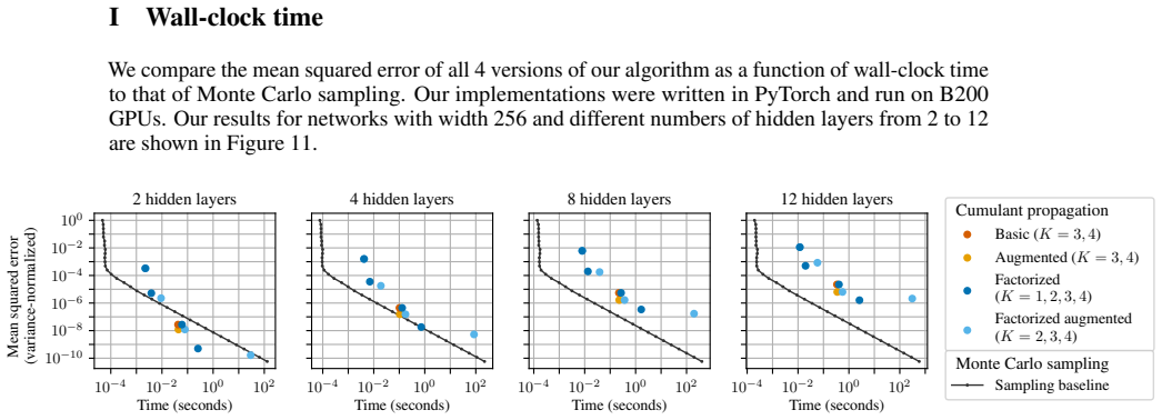
Mean over 5 random seeds shown. (Error bars hidden because they would be too small to be readable.) In most cases, our algorithms underperform sampling. This appears to be largely because our algorithms spend the majority of the wall-clock time on a small fraction of the FLOPs that are implemented inefficiently in pure Python. In addition, they perform a ...
work page 2015
-
[10]
This is our main result, Theorem S.2.15
Tracking the cumulants listed above does indeed produce MSE O(n−K). This is our main result, Theorem S.2.15
-
[11]
Tracking these cumulants takes time O(nK+1). This is easily verified during the description of the algorithm in Sections S.2.6 and S.4. Note that for this analysis to hold, we require that K is bounded above by a constant. This is exactly where the requirement thatε(n)is noticeable comes from. Let us now look at each stage of the algorithms in more detail...
-
[12]
We can explicitly sum this infinite collection ofΘ(1) terms. By the orthogonality property for Hermite polynomials, cϕ2Z 0 =E[ϕ 2] =E ∞X k1,k2=0 σk1+k2 k1!k2! bϕZ k1 bϕZ k2Hek1 σ−1Z Hek2 σ−1Z = ∞X k=0 1 k! bϕZ k 2 σ2k and so κ2[ϕ(Z)] i,i =cϕ2Z 0 −(bϕZ 0 )2. We can always do this summation to remove the Θ(1) terms in (5) when indices are repeated.17
-
[13]
Alternatively, by writing the cumulant in terms of expectations and collecting equal indices, we can write any cumulant as a polynomial in cumulants of powers with pairwise distinct indices. For example, κ2[ϕ(Z)] i,i =κ 1[ϕ2(Z)] i −κ 1[ϕ(Z)]2 i κ3[ϕ(Z)] i,i,j =κ 2[ϕ2(Z), ϕ(Z)] i,j −2κ 2[ϕ(Z)] i,jκ1[ϕ(Z)] i. We call this constructionpower cumulants(see Sec...
work page 2013
-
[14]
For eachv∈V 1,T v is a symmetric tensor sequence withdeg(v) = rank(T v). Let rank(D) :=|V 2 \I| . Call D connectedif BD is connected; call itfully-contractedif rank(D) =
-
[15]
We say the diagramDisat layerℓif every tensor sequence is at layerℓ. This should be interpreted as an einsum in the following way: the vertices v∈V 2 correspond to indices, those in I are contracted indices, those not in I are “hanging" indices, and the tensor diagram corresponds to a tensor sequence where the contracted indices have been summed over, giv...
-
[16]
Forr∈[R], initialize tensors ˜ηr[X(0)] :=h ≤r−2sK(r)(κr[X(0)]) = 1r= 2andK= 1 In r= 2andK >1 0r̸= 2
-
[17]
For1≤ℓ≤L, repeat the following: (a) Compute the tensors T(ℓ) r := ˜ηr[X(ℓ−1)]⊙W (ℓ) ∀r∈[R] M(ℓ) i,j := (W(ℓ)W(ℓ)⊤)i,j K >1ori=j 0otherwise. Note that each T(ℓ) r is a symmetric contraction of a (r−2s K(r))-tensor, and thus takes time O(nr−2sK(r)+1)≤O(n K+1). The matrix M(ℓ) takes time O(n2) if K= 1 and otherwise O(n3). In any case, this is no more than th...
-
[18]
ReturnW (L+1)˜η1[X(L)]. S.2.7 Error analysis In this section, we prove that the polynomial algorithm described above satisfies the conditions of Theorem 5.1. Define the error tensors ∆r[X(ℓ)] :=κ r[X(ℓ)]−˜κr[X(ℓ)] ∆r[Z(ℓ)] :=κ r[Z(ℓ)]−˜κr[Z(ℓ)] These are tensor sequences. Our main result is the following theorem: Theorem S.2.15.For all r≥1 and ℓ∈[L+ 1] , ...
work page 2015
-
[19]
Initialize tensors ˜ηr[X(0)] =h ≥r−2sK(r)(κr[X(0)]) = 1r= 2andK= 1 In r= 2andK >1 0r̸= 2
-
[20]
For1≤ℓ≤L, repeat the following: (a) Compute the tensors T(ℓ) r := ˜ηr[X(ℓ−1)]⊙W (ℓ) ∀r∈[R] M(ℓ) := D(2)(W(ℓ)W(ℓ)⊤)K= 1 W(ℓ)W(ℓ)⊤ K >1. Note that each T(ℓ) r is a symmetric contraction of a (r−2s K(r))-tensor, and thus takes time O(nr−2sK(r)+1)≤O(n K+1). The matrix M(ℓ) takes time O(n2) if K= 1 , otherwise O(n3). In any case, this is no more than theO(n K+...
-
[21]
ReturnW (L+1)˜η1[X(L)]. S.4.2 Augmented algorithm The basic algorithm in Section S.4.1 works by tracking every harmonic part that would incur at least Ω(n−K+1) MSE if dropped; the largest of these parts takes Θ(nK+1) time to propagate. We may consider an algorithm that additionally tracks every harmonic part that can be propagated in O(nK) time and contri...
-
[22]
for allk 0 ≥0,r≥1andα ∈Z r ≥1, the tensor sequence RP α,k0 [ϕ(Z)] j1,...,jr := 1(j1, ..., jr distinct) · κP α[ϕ(Z)]− X k∈Zr ≥0 |k|≤k0 1 k! rY a=1 dϕαa (E[Z],Var[Z]) ka ja X π∈cDia[≤2](k) Y S∈π κ[Z jv : (v, w)∈S] 52 hasn − k0 +1 4 -growth
-
[23]
For anyα, k≥0, the rank-1tensor sequences cϕα(E[Z],Var[Z]) k haveO(1)-growth
-
[24]
We prove that polynomials are tame with respect to Z(ℓ) in Section S.5.3
If µ, σ2 ∈R n are rank-1 tensor sequences such that E[Z]−µ and Var[Z]−σ 2 have n−k0-growth, then ∆cϕαk :=cϕα(E[Z],Var[Z]) k −cϕα(µ,σ2) k hasn −k0-growth. We prove that polynomials are tame with respect to Z(ℓ) in Section S.5.3. Our main result is the following theorem, which does not assume that the activation functions are polynomials: Theorem S.5.2.Supp...
-
[25]
for allℓ∈[L],ϕ ℓ is tame with respect toZ (ℓ); and
-
[26]
for all ℓ∈[L+ 1] , the conclusion of Proposition S.2.12 holds: connected fully-contracted diagrams of (pre-)activation cumulants haven-growth. Then, for allr≥1andℓ∈[L+ 1], the tensor sequence∆ r[Z(ℓ)]hasn −(K/2) growth. As stated, we are focusing just on the basic algorithm (the error of the factorized algorithm is precisely the same, the only difference ...
work page 1992
discussion (0)
Sign in with ORCID, Apple, or X to comment. Anyone can read and Pith papers without signing in.