Effective Hamiltonians in Cavity and Waveguide QED from Transition-Operator Diagrammatic Perturbation Theory
Pith reviewed 2026-05-15 05:18 UTC · model grok-4.3
The pith
Transition-operator diagrammatic perturbation theory enables systematic derivation of effective Hamiltonians in cavity and waveguide QED at arbitrary orders.
A machine-rendered reading of the paper's core claim, the machinery that carries it, and where it could break.
Core claim
The authors propose an adiabatic-elimination formalism in the dispersive regime based on a transition-centric perturbation theory. The perturbative expansion is recast into a diagrammatic framework, while adiabatic elimination is implemented through controlled projections onto transition subspaces. This yields effective higher-order Hamiltonians for multilevel systems and multiple qubits in cavity and waveguide quantum electrodynamics.
What carries the argument
Transition-operator diagrammatic perturbation theory combined with controlled projections onto transition subspaces to perform adiabatic elimination.
If this is right
- Effective Hamiltonians become constructible at any perturbation order without accumulating uncontrolled errors.
- The same framework covers both cavity and waveguide geometries for arbitrary numbers of qubits or atomic levels.
- Multiphoton processes in the dispersive regime receive systematic, explicit corrections beyond second order.
- Existing limitations on system complexity or perturbative order are bypassed for concrete calculations.
Where Pith is reading between the lines
- The method could be tested by comparing predicted fourth-order shifts against exact diagonalization in small systems.
- Time-dependent drives or weak dissipation might be incorporated by extending the same diagrammatic rules.
- Similar transition-operator projections could simplify effective models in circuit QED or Rydberg arrays.
Load-bearing premise
The perturbative expansion and the projections onto transition subspaces remain valid and controlled at arbitrary orders in the dispersive regime.
What would settle it
A measured higher-order dispersive shift or multiphoton transition rate in a two-qubit or multilevel system that deviates from the explicit effective Hamiltonian constructed by the method.
Figures


read the original abstract
We propose an adiabatic-elimination formalism in the dispersive regime based on a transition-centric perturbation theory. The perturbative expansion is recast into a diagrammatic framework, while adiabatic elimination is implemented through controlled projections onto transition subspaces. Our approach applies systematically at arbitrary perturbation order, and is suited to multilevel systems and multiple qubits in both cavity and waveguide quantum electrodynamics. It ultimately enables the explicit construction of effective higher-order Hamiltonians while bypassing important limitations of existing techniques, thereby providing a practical toolbox for multiphoton processes in the dispersive regime.
Editorial analysis
A structured set of objections, weighed in public.
Referee Report
Summary. The paper proposes a transition-centric diagrammatic perturbation theory for adiabatic elimination in the dispersive regime of cavity and waveguide QED. It recasts the perturbative expansion into diagrams and implements elimination through controlled projections onto transition subspaces, enabling systematic construction of effective Hamiltonians at arbitrary orders for multilevel systems and multiple qubits while bypassing limitations of prior methods.
Significance. If the projection rules and diagrammatic construction hold, the approach supplies a practical, order-by-order toolbox for higher-order effective Hamiltonians in multi-qubit and multilevel dispersive systems. The systematic character at arbitrary perturbation order and explicit applicability to both cavity and waveguide geometries constitute a clear advance over existing adiabatic-elimination techniques that often require case-by-case fitting or truncation.
minor comments (3)
- The abstract states that the method 'bypasses important limitations of existing techniques,' but the manuscript should include a concise table or paragraph in the introduction that explicitly lists those limitations (e.g., restriction to two-level systems, inability to reach third-order terms) and shows how the diagrammatic projection rules overcome each one.
- Notation for the transition operators and the projection rules onto subspaces should be introduced with a single, self-contained definition block early in the text (ideally §2) rather than being distributed across multiple sections; this would improve readability for readers unfamiliar with the diagrammatic formalism.
- The manuscript would benefit from at least one fully worked numerical example (e.g., a three-level atom coupled to a waveguide) that compares the derived effective Hamiltonian against exact diagonalization or master-equation simulation up to the claimed perturbative order.
Simulated Author's Rebuttal
We thank the referee for their positive assessment of the manuscript, including the recognition of its systematic character at arbitrary order and applicability to both cavity and waveguide geometries. We appreciate the recommendation for minor revision.
Circularity Check
No significant circularity detected
full rationale
The derivation chain consists of a standard perturbative expansion in the dispersive regime, recast into a diagrammatic representation with explicit projection rules onto transition subspaces. These steps are defined directly from the system Hamiltonian and the adiabatic-elimination condition without invoking fitted parameters, self-referential definitions, or load-bearing self-citations. The resulting effective Hamiltonians at arbitrary order follow from the diagrammatic rules applied to the original interaction terms, remaining self-contained and independent of the target result.
Axiom & Free-Parameter Ledger
axioms (2)
- domain assumption The system operates in the dispersive regime where detuning greatly exceeds coupling strengths.
- domain assumption Perturbation theory converges at arbitrary order for the targeted multilevel and multi-qubit systems.
Reference graph
Works this paper leans on
-
[1]
Recall the perturbative expansion Eq
Computation with nested convolution products We first carry out the calculation by means of nested convolution products arising from the perturbative expansion. Recall the perturbative expansion Eq. (15) ˆξj(0) iσ (ω, t) =e −iLfree(t−t0) ˆξj iσ(ω) (B1) ˆξj(1) iσ (ω, t) =−i Z t t0 dτ e −iLfree(t−τ) Linte−iLfree(τ−t 0) ˆξj iσ(ω) (B2) ˆξj(2) iσ (ω, t) = (−i)...
-
[2]
Computation with the resolvent In this subsection, we demonstrate how the time weightsv n(t) in Eq. (B13) may equivalently be retrieved by manipulating the resolventG(s) of the LiouvillianL G(s) = 1 s+iL ,Re(s)>0.(B14) G(s) is obtained by considering the evolution superoperator in Liouville spaceU(t, t 0) =e −iL(t−t0) define as dU(t, t 0) dt =−iL U(t, t 0...
-
[3]
Computation of the reverse process’ weight This section provides a computation of the time weightv reverse n (t) of the reverse process of a givenn-th order JLM transition operator of time weightv n(t), which reads vn(t) = (−1)NL nX l=0 e−i∆lte−Θlt nY k=0 k̸=l 1 ∆l −∆ k +i(Θ k −Θ l) (B20) More specifically, we show thatv reverse n (t) =v ∗ n(t), entailing...
-
[4]
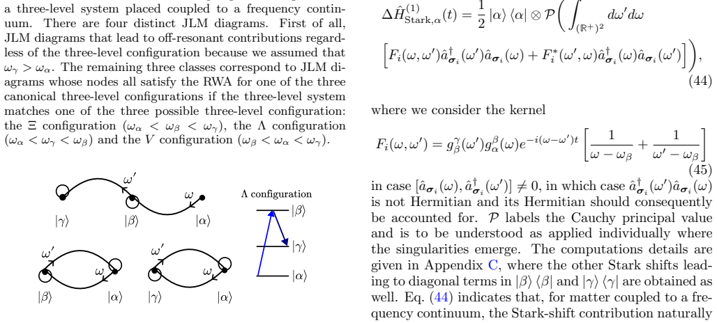
1 (t)|γ⟩ ⟨α| ⊗ˆa† σj(ω′)ˆaσi(ω) + h.c,(C4) where the 1/2 factor stems from rule (R5) II B
Mediated-coupling correction The correction to the interaction Hamiltonian due to the mediated coupling|γ⟩ ⟨α| ⊗ˆa † σj(ω′)ˆaσi(ω) reads ∆ ˆH(1) med.(t) = 1 2 Z R+ dω g β α(ω) Z R+ dω′ gγ β(ω′)W total,med. 1 (t)|γ⟩ ⟨α| ⊗ˆa† σj(ω′)ˆaσi(ω) + h.c,(C4) where the 1/2 factor stems from rule (R5) II B. Using Eq. (C3), ∆ ˆH(1) med.(t) = 1 2 Z R+ dω g β α(ω) Z R+ ...
-
[5]
Stark-shift correction Employing the same procedure for the Stark-shift contributions lead to the total correction to the Hamiltonian at first order ∆ ˆH(1) int (t) ∆ ˆH(1) int (t) = 1 2 |γ⟩ ⟨α| ⊗ P Z (R+)2 dω′dω g γ β(ω′)gβ α(ω)e−i(ω−ω ′−ωγ)t 1 δi(ω) − 1 δj(ω′) ˆa† σj(ω′)ˆaσi(ω) ! + h.c + 1 2 |α⟩ ⟨α| ⊗ P Z (R+)2 dω′dω h Fi(ω, ω′)ˆa† σi(ω′)ˆaσi(ω) +F ∗ i ...
-
[6]
Consider the interaction Hamiltonian Eq
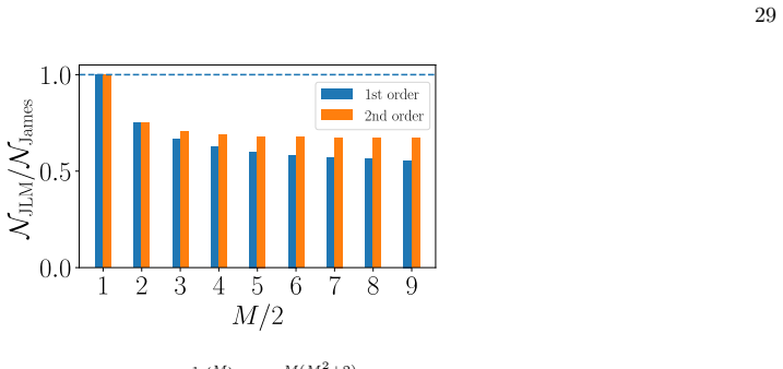
Combinatorial upper bound This section is dedicated to evaluating the number of JLM diagrams needed to encapsulate the whole system’s dynamics. Consider the interaction Hamiltonian Eq. (3) in a more compact form Eq. (4) with a numberMof JLM transition operators ˆHint =PM/2 m=1 ˆξm + h.c where ˆξm are the zeroth-order JLM transition operators. a. Multileve...
-
[7]
JLM diagrams multiplicities In this subsection, we illustrate, for a multilevel atomic system, the matter-cyclic condition and the role of bosonic- operator permutations for first- and second-order JLM diagrams. For simplicity and without loss of generality, the bosonic modes are defined for a discrete set, not a continuum. a. First order Consider a first...
-
[8]
Number of JLM diagrams This subsection is dedicated to calculating an upper limit on the number of JLM diagrams to be drawn at first and second order of the perturbation expansion. a. First order At first ordern= 1 of the perturbation expansion, the previous section demonstrated thatat most M+1 2 JLM diagrams – which correspond toat most4 M+1 2 first-orde...
-
[9]
Weight computation In this subsection, we compute the weightV 2(t) of the second-order three-photon JLM diagrams. As before, V2(t) denotes the time-dependent contribution ofW 2(t) which also accounts for the coupling terms involved in the corresponding diagram. Recalling the general canonical time weight Eq. (20) atnth order of a givennth order JLM transi...
-
[10]
Dealing with cumulative-detuning degeneracies As opposed to the first-order computation covered in Sec. II B 7, poles may emerge ifδ j =−δ k,δ j =−δ i or δk =δ i =−δ j, which amounts to having cumulative-detuning degeneracies ∆ 0 = ∆ 2. We now show that the divergences cancel. Let us assume for instance thatδ j =−δ k and analyzev canonical 2 (t) where a p...
-
[11]
H.-P. Breuer and F. Petruccione,The theory of open quantum systems(OUP Oxford, 2002)
work page 2002
-
[12]
D. Finkelstein-Shapiro, D. Viennot, I. Saideh, T. Hansen, T. Pullerits, and A. Keller, Adiabatic elimination and subspace evolution of open quantum systems, Physical Review A101, 042102 (2020)
work page 2020
-
[13]
C. Gonzalez-Ballestero, Tutorial: projector approach to master equations for open quantum systems, Quantum8, 1454 (2024)
work page 2024
-
[14]
F.-M. Le R´ egent and P. Rouchon, Heisenberg formulation of adiabatic elimination for open quantum systems with two timescales, in2023 62nd IEEE Conference on Decision and Control (CDC)(IEEE, 2023) pp. 7208–7213
work page 2023
-
[15]
R. Puri and R. Bullough, Quantum electrodynamics of an atom making two-photon transitions in an ideal cavity, Journal of the Optical Society of America B5, 2021 (1988)
work page 2021
-
[16]
C. C. Gerry and J. Eberly, Dynamics of a raman coupled model interacting with two quantized cavity fields, Physical Review A42, 6805 (1990)
work page 1990
-
[17]
Y. Wu, Effective raman theory for a three-level atom in theλconfiguration, Physical Review A54, 1586 (1996)
work page 1996
-
[18]
M. Alexanian and S. K. Bose, Unitary transformation and the dynamics of a three-level atom interacting with two quantized field modes, Physical Review A52, 2218 (1995)
work page 1995
- [19]
-
[20]
V. Paulisch, H. Rui, H. K. Ng, and B.-G. Englert, Beyond adiabatic elimination: A hierarchy of approximations for multi-photon processes, The European Physical Journal Plus129, 1 (2014)
work page 2014
-
[22]
P. Maity, Adiabatic elimination in the presence of multiphoton transitions in atoms inside a cavity, International Journal of Modern Physics B , 2450439 (2024)
work page 2024
-
[23]
J. Pedernales, I. Lizuain, S. Felicetti, G. Romero, L. Lamata, and E. Solano, Quantum rabi model with trapped ions, Scientific reports5, 15472 (2015)
work page 2015
-
[24]
A. Linskens, I. Holleman, N. Dam, and J. Reuss, Two-photon rabi oscillations, Physical Review A54, 4854 (1996)
work page 1996
- [25]
-
[26]
D. James and J. Jerke, Effective hamiltonian theory and its applications in quantum information, Canadian Journal of Physics85, 625 (2007)
work page 2007
-
[27]
O. Gamel and D. F. James, Time-averaged quantum dynamics and the validity of the effective hamiltonian model, Physical Review A—Atomic, Molecular, and Optical Physics82, 052106 (2010)
work page 2010
-
[28]
N. N. Bogolubov Jr, A. K. Prykarpatsky, and U. Taneri,Quantum field theory with application to quantum nonlinear optics (World Scientific Publishing Company, 2002)
work page 2002
-
[29]
Zee,Quantum field theory in a nutshell, Vol
A. Zee,Quantum field theory in a nutshell, Vol. 7 (Princeton university press, 2010). 33
work page 2010
-
[30]
C. J. Bord´ e, Density matrix equations and diagrams for high resolution non-linear laser spectroscopy: application to ramsey fringes in the optical domain, inAdvances in laser spectroscopy(Springer, 1983) pp. 1–70
work page 1983
-
[31]
R. W. Boyd, A. L. Gaeta, and E. Giese, Nonlinear optics, inSpringer Handbook of Atomic, Molecular, and Optical Physics (Springer, 2008) pp. 1097–1110
work page 2008
-
[32]
Hache,Optique non lin´ eaire(EDP Sciences Les Ulis, France, 2016)
F. Hache,Optique non lin´ eaire(EDP Sciences Les Ulis, France, 2016)
work page 2016
-
[33]
C. A. Marx, U. Harbola, and S. Mukamel, Nonlinear optical spectroscopy of single, few, and many molecules: Nonequilib- rium green’s function qed approach, Physical Review A—Atomic, Molecular, and Optical Physics77, 022110 (2008)
work page 2008
-
[34]
O. Roslyak and S. Mukamel, A unified description of sum frequency generation, parametric down conversion and two-photon fluorescence, Molecular physics107, 265 (2009)
work page 2009
-
[35]
S. Mukamel and S. Rahav, Ultrafast nonlinear optical signals viewed from the molecule’s perspective: Kramers–heisenberg transition-amplitudes versus susceptibilities, inAdvances in atomic, molecular, and optical physics, Vol. 59 (Elsevier, 2010) pp. 223–263
work page 2010
-
[36]
K. E. Dorfman, F. Schlawin, and S. Mukamel, Nonlinear optical signals and spectroscopy with quantum light, Rev. Mod. Phys.88, 045008 (2016)
work page 2016
-
[37]
M. A. Marques and E. K. Gross, Time-dependent density functional theory, Annu. Rev. Phys. Chem.55, 427 (2004)
work page 2004
-
[38]
F. Vergari, F. Mazza, A. Hosseinnia, and M. Marrocco, Diagrammatic schemes for nonlinear optical interactions, Journal of Raman Spectroscopy (2025)
work page 2025
-
[39]
S. Mukamel,Principles of nonlinear optical spectroscopy, Oxford series in optical and imaging sciences (Oxford University Press, 1995)
work page 1995
-
[40]
R. Sutherland and R. Srinivas, Universal hybrid quantum computing in trapped ions, Physical Review A104, 032609 (2021)
work page 2021
-
[41]
J. Ackerhalt and K. Rza˙ zewski, Heisenberg-picture operator perturbation theory, Physical Review A12, 2549 (1975)
work page 1975
-
[42]
J. Franson and M. M. Donegan, Perturbation theory for quantum-mechanical observables, Physical Review A65, 052107 (2002)
work page 2002
-
[43]
F. M. Fern´ andez, Perturbation theory for heisenberg operators, Physical Review A67, 022104 (2003)
work page 2003
-
[44]
A. Blais, R.-S. Huang, A. Wallraff, S. M. Girvin, and R. J. Schoelkopf, Cavity quantum electrodynamics for superconducting electrical circuits: An architecture for quantum computation, Physical Review A—Atomic, Molecular, and Optical Physics 69, 062320 (2004)
work page 2004
-
[45]
R. H. Dicke, Coherence in spontaneous radiation processes, Physical review93, 99 (1954)
work page 1954
-
[46]
J. Larson and T. Mavrogordatos,The Jaynes–Cummings model and its descendants: modern research directions(IoP Publishing, 2021)
work page 2021
-
[47]
M. Meguebel, M. Federico, L. Garbe, N. Belabas, and N. Fabre, Transitions as the native objects of dispersive light-matter dynamics, (2026)
work page 2026
-
[48]
J. A. Gyamfi, Fundamentals of quantum mechanics in liouville space, European Journal of Physics41, 063002 (2020)
work page 2020
-
[49]
J. J. Sakurai and J. Napolitano,Modern quantum mechanics(Cambridge University Press, 2020)
work page 2020
-
[50]
B. C. Hall,Quantum theory for mathematicians(Springer, 2013)
work page 2013
-
[51]
C. Cohen-Tannoudji, J. Dupont-Roc, and G. Grynberg,Atom-photon interactions: basic processes and applications(John Wiley & Sons, 2024)
work page 2024
-
[52]
F. Bloch and A. Siegert, Magnetic resonance for nonrotating fields, Physical Review57, 522 (1940)
work page 1940
-
[53]
P. Forn-D´ ıaz, J. Lisenfeld, D. Marcos, J. J. Garc´ ıa-Ripoll, E. Solano, C. J. P. M. Harmans, and J. E. Mooij, Observation of the bloch-siegert shift in a qubit-oscillator system in the ultrastrong coupling regime, Phys. Rev. Lett.105, 237001 (2010)
work page 2010
-
[54]
K. K. Ma and C. Law, Three-photon resonance and adiabatic passage in the large-detuning rabi model, Physical Review A92, 023842 (2015)
work page 2015
-
[55]
Q. Xie, H. Zhong, M. T. Batchelor, and C. Lee, The quantum rabi model: solution and dynamics, Journal of Physics A: Mathematical and Theoretical50, 113001 (2017)
work page 2017
- [56]
- [57]
-
[58]
M. Ayyash and S. Ashhab, Dispersive regime of multiphoton qubit-oscillator interactions, Physical Review A112, 023713 (2025)
work page 2025
-
[59]
P. M. Chaikin, T. C. Lubensky, and T. A. Witten,Principles of condensed matter physics, Vol. 10 (Cambridge university press Cambridge, 1995)
work page 1995
-
[60]
J. Lepp¨ akangas, J. Braum¨ uller, M. Hauck, J.-M. Reiner, I. Schwenk, S. Zanker, L. Fritz, A. V. Ustinov, M. Weides, and M. Marthaler, Quantum simulation of the spin-boson model with a microwave circuit, Physical Review A97, 052321 (2018)
work page 2018
-
[61]
A. Parra-Rodriguez, E. Rico, E. Solano, and I. Egusquiza, Quantum networks in divergence-free circuit qed, Quantum Science and Technology3, 024012 (2018)
work page 2018
-
[62]
M. Meguebel, M. Federico, S. Felicetti, N. Belabas, and N. Fabre, Generation of frequency entanglement with an effective quantum dot-waveguide two-photon quadratic interaction, Optica Quantum3, 617 (2025)
work page 2025
- [63]
-
[64]
S. Gu´ erin and H.-R. Jauslin, Control of quantum dynamics by laser pulses: Adiabatic floquet theory, Advances in Chemical Physics125, 147 (2003). 34
work page 2003
-
[65]
A. J. Leggett, S. Chakravarty, A. T. Dorsey, M. P. Fisher, A. Garg, and W. Zwerger, Dynamics of the dissipative two-state system, Reviews of Modern Physics59, 1 (1987)
work page 1987
-
[66]
J. J. G. Ripoll,Quantum information and quantum optics with superconducting circuits(Cambridge University Press, 2022)
work page 2022
-
[67]
O. Bazavan, S. Saner, D. Webb, E. Ainley, P. Drmota, D. Nadlinger, G. Araneda, D. Lucas, C. Ballance, and R. Srinivas, Squeezing, trisqueezing, and quadsqueezing in a spin-oscillator system (2024), arXiv preprint arXiv:2403.05471
-
[68]
Appel,Math´ ematiques pour la physique et les physiciens(H & K, 2002)
W. Appel,Math´ ematiques pour la physique et les physiciens(H & K, 2002)
work page 2002
-
[69]
KREYSZIG, Advanced engineering mathematics (2021)
E. KREYSZIG, Advanced engineering mathematics (2021)
work page 2021
-
[70]
P. Blanchard and E. Br¨ uning,Mathematical methods in Physics: Distributions, Hilbert space operators, variational methods, and applications in quantum physics, Vol. 69 (Birkh¨ auser, 2015)
work page 2015
-
[71]
W. Shao, C. Wu, and X.-L. Feng, Generalized james’ effective hamiltonian method, Physical Review A95, 032124 (2017)
work page 2017
-
[72]
generalized james’ effective hamiltonian method
W. Rosado and I. Arraut, Comment on “generalized james’ effective hamiltonian method”, Physical Review A108, 066201 (2023)
work page 2023
-
[73]
J. C. Garrison and R. Y. Chiao,Quantum Optics(Oxford University Press, 2014)
work page 2014
discussion (0)
Sign in with ORCID, Apple, or X to comment. Anyone can read and Pith papers without signing in.