GraphMAR: Geometry-Aware Graph Learning Framework for Spatially Adaptive CT Metal Artifact Reduction
Pith reviewed 2026-05-20 13:56 UTC · model grok-4.3
The pith
GraphMAR aligns routing maps with geometric density graphs from metal masks to localize and reduce CT artifacts in the image domain
A machine-rendered reading of the paper's core claim, the machinery that carries it, and where it could break.
Core claim
The paper claims that a geometric density graph constructed from the metal mask in the reconstructed image serves as a workable image-domain stand-in for sinogram metal traces, enabling a GraphMoE module to build a polar-coordinate artifact graph in feature space, route experts adaptively across regions, and produce explicit localization by aligning learned routing maps with the geometric prior.
What carries the argument
The geometric density graph derived from inter-implant geometry in the metal mask, which localizes artifact-prone regions, together with GraphMoE, the graph-routed mixture-of-experts module that builds a polar-coordinate artifact graph to adaptively assign experts to different spatial regions.
If this is right
- Region-adaptive processing yields higher restoration quality than uniform image-domain methods on both simulated and real-world datasets.
- Alignment of routing maps with the geometric density graph supplies explicit, interpretable artifact localization in the image domain.
- The framework operates without raw sinogram data, making it applicable to standard clinical reconstructed images.
- Graph-based modeling introduces a new mechanism for handling spatially varying artifact patterns induced by multiple implants.
Where Pith is reading between the lines
- The same mask-to-graph construction could be tested on artifacts from non-metallic high-density objects such as bone or contrast agents.
- Routing maps produced by the method could serve as attention priors for other downstream tasks like segmentation in metal-affected regions.
- Extending the polar-coordinate artifact graph to include temporal information might support correction in dynamic or 4D CT acquisitions.
Load-bearing premise
A geometric graph built solely from the metal mask in the reconstructed image can reliably identify artifact-prone regions without access to the original projection measurements.
What would settle it
A test set of real CT scans with precisely measured metal implant positions where the geometric density graph shows no correspondence to the actual locations or severity of streaking artifacts after reconstruction.
Figures


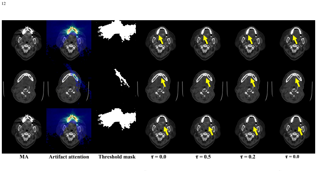
read the original abstract
Computed tomography (CT) metal artifact reduction (MAR) aims to reduce the severe streaking artifacts induced by metallic implants and other high-density objects. Effective MAR generally requires both accurate artifact localization and artifact removal. Sinogram-domain methods can exploit explicit geometric cues, such as metal traces, to identify metal-corrupted measurements, while requiring raw projection data, which is often unavailable in clinical and practical scenarios. Image-domain methods are more flexible and widely applicable, yet they usually lack comparable geometric guidance, limiting their ability to localize artifacts and leading to suboptimal results. To address this limitation, we propose GraphMAR, a geometry-aware learning framework for explicit artifact identification and spatially adaptive MAR in the image domain. The key idea is to introduce graph-based geometric modeling as an image-domain analogue of sinogram metal traces. Specifically, we first construct a geometric graph from the metal mask and derive a geometric density graph that coarsely localizes artifact-prone regions according to inter-implant geometry. We then design GraphMoE, a graph-routed mixture-of-experts module that builds a polar-coordinate artifact graph in feature space and adaptively routes different experts to different spatial regions for MAR. By aligning the learned routing maps with the geometric density graph, GraphMAR provides explicit and interpretable artifact localization while enabling region-adaptive artifact reduction. Experiments on both simulated and real-world datasets demonstrate that GraphMAR achieves superior MAR performance compared with existing methods. To the best of our knowledge, this is the first work to introduce graph-based modeling for CT MAR and to enable explicit artifact identification in the image domain, improving both restoration quality and interpretability.
Editorial analysis
A structured set of objections, weighed in public.
Referee Report
Summary. The manuscript proposes GraphMAR, a geometry-aware graph learning framework for CT metal artifact reduction (MAR) in the image domain. It constructs a geometric density graph from the metal mask to localize artifact-prone regions based on inter-implant geometry and introduces the GraphMoE module, which builds a polar-coordinate artifact graph in feature space to adaptively route experts for region-specific artifact reduction. By aligning learned routing maps with the geometric density graph, the method aims to provide explicit and interpretable artifact localization. Experiments on simulated and real-world datasets are claimed to show superior performance over existing methods, positioning it as the first graph-based approach for CT MAR.
Significance. If the results hold, this work could significantly advance image-domain MAR by providing a geometric modeling approach that mimics sinogram-domain cues without needing raw projection data. The explicit interpretability through routing maps aligned with geometric density is a strength, potentially improving both restoration quality and clinical trust. The introduction of graph-based modeling and GraphMoE for adaptive processing represents a novel direction in the field.
major comments (1)
- [Abstract and §3] Abstract and §3 (geometric density graph construction): The assumption that a geometric density graph built solely from the metal mask in the reconstructed image serves as a reliable image-domain analogue to sinogram metal traces is load-bearing for the central claim of explicit and interpretable artifact localization. Artifact streaks arise from specific ray paths under CT geometry and polychromatic spectrum; the image-domain graph using only inter-implant distances or densities omits scanner angles, source-detector geometry, and attenuation coefficients. This is least secure for multi-implant or off-center cases, as highlighted by the stress-test concern. A direct validation (e.g., overlap with ground-truth artifact maps from projection data or ablation across implant configurations) is needed to support the claim.
minor comments (2)
- [Abstract] Abstract: The statement 'to the best of our knowledge, this is the first work to introduce graph-based modeling for CT MAR' requires a more exhaustive related-work discussion to substantiate novelty.
- [Experiments] Experiments section: Claims of superior performance should include specific quantitative metrics (e.g., PSNR, SSIM), error bars, statistical significance tests, and ablation studies on the geometric density graph and GraphMoE components.
Simulated Author's Rebuttal
We thank the referee for the positive assessment of our work and the constructive major comment. We address the concern regarding the geometric density graph point by point below.
read point-by-point responses
-
Referee: [Abstract and §3] Abstract and §3 (geometric density graph construction): The assumption that a geometric density graph built solely from the metal mask in the reconstructed image serves as a reliable image-domain analogue to sinogram metal traces is load-bearing for the central claim of explicit and interpretable artifact localization. Artifact streaks arise from specific ray paths under CT geometry and polychromatic spectrum; the image-domain graph using only inter-implant distances or densities omits scanner angles, source-detector geometry, and attenuation coefficients. This is least secure for multi-implant or off-center cases, as highlighted by the stress-test concern. A direct validation (e.g., overlap with ground-truth artifact maps from projection data or ablation across implant configurations) is needed to support the claim.
Authors: We thank the referee for this insightful observation. We agree that the geometric density graph is an approximation that encodes inter-implant geometry from the metal mask but does not explicitly incorporate scanner angles, source-detector geometry, or polychromatic effects. Our design choice is motivated by the fact that, in the image domain, streaking artifacts predominantly manifest along paths connecting high-density implants, which the graph structure directly captures via distances and densities. Nevertheless, to strengthen the central claim of explicit localization, we will revise the manuscript to include additional validation experiments on the simulated datasets. These will report quantitative overlap (e.g., Dice or IoU) between the geometric density graph and ground-truth artifact maps derived from projection data, together with ablations across multi-implant and off-center configurations. We believe this will provide the requested direct evidence while preserving the method's applicability to real-world image-only scenarios. revision: yes
Circularity Check
No significant circularity detected in derivation chain
full rationale
The paper introduces novel components including a geometric density graph constructed from the metal mask, a polar-coordinate artifact graph, and the GraphMoE module. These are defined from the input metal mask and inter-implant geometry without reducing to fitted target quantities or prior self-citations by construction. The central claims rest on explicit modeling choices and experimental results rather than tautological redefinitions or load-bearing self-citations. This is a standard case of a self-contained proposal against external benchmarks.
Axiom & Free-Parameter Ledger
axioms (1)
- domain assumption A geometric graph derived from the metal mask can coarsely localize artifact-prone regions according to inter-implant geometry
invented entities (2)
-
geometric density graph
no independent evidence
-
GraphMoE module
no independent evidence
Lean theorems connected to this paper
-
IndisputableMonolith/Cost/FunctionalEquation.leanwashburn_uniqueness_aczel unclear?
unclearRelation between the paper passage and the cited Recognition theorem.
we first construct a geometric graph from the metal mask and derive a geometric density graph that coarsely localizes artifact-prone regions according to inter-implant geometry... polar-coordinate artifact graph... angular edges... radial edges... L_graph = ||Norm(GA)−Norm(G)||_2^2
-
IndisputableMonolith/Foundation/AlexanderDuality.leanalexander_duality_circle_linking unclear?
unclearRelation between the paper passage and the cited Recognition theorem.
GraphMAR... first work to introduce graph-based modeling for CT MAR
What do these tags mean?
- matches
- The paper's claim is directly supported by a theorem in the formal canon.
- supports
- The theorem supports part of the paper's argument, but the paper may add assumptions or extra steps.
- extends
- The paper goes beyond the formal theorem; the theorem is a base layer rather than the whole result.
- uses
- The paper appears to rely on the theorem as machinery.
- contradicts
- The paper's claim conflicts with a theorem or certificate in the canon.
- unclear
- Pith found a possible connection, but the passage is too broad, indirect, or ambiguous to say the theorem truly supports the claim.
Reference graph
Works this paper leans on
-
[1]
Metal artifact reduction in CT: where are we after four decades?
L. Gjestebyet al., “Metal artifact reduction in CT: where are we after four decades?”IEEE Access, vol. 4, pp. 5826–5849, 2016
work page 2016
-
[2]
Aapm ct metal artifact reduction grand challenge,
E. Haneda, N. Peters, J. Zhang, G. Karageorgos, W. Xia, H. Paganetti, G. Wang, Y . Guo, J. Ma, H. S. Park, K. Jeon, F. Fan, M. Thies, and B. De Man, “Aapm ct metal artifact reduction grand challenge,”Medical Physics, vol. 52, no. 10, p. e70050, 2025
work page 2025
-
[3]
Deep sinogram completion with image prior for metal artifact reduction in CT images,
L. Yu, Z. Zhang, X. Li, and L. Xing, “Deep sinogram completion with image prior for metal artifact reduction in CT images,”IEEE Trans. Med. Imaging, vol. 40, no. 1, pp. 228–238, 2020
work page 2020
-
[4]
DuDoNet: Dual domain network for CT metal artifact reduction,
W.-A. Linet al., “DuDoNet: Dual domain network for CT metal artifact reduction,” inProc. IEEE Conf. Comput. Vis. Pattern Recognit., 2019, pp. 10 512–10 521
work page 2019
-
[5]
Encoding metal mask projection for metal artifact reduction in computed tomography,
Y . Lyu, W.-A. Lin, H. Liao, J. Lu, and S. K. Zhou, “Encoding metal mask projection for metal artifact reduction in computed tomography,” inProc. Int. Conf. Med. Image Comput. Comput.-Assisted Intervention, 2020, pp. 147–157
work page 2020
-
[6]
InDuDoNet: An interpretable dual domain network for CT metal artifact reduction,
H. Wanget al., “InDuDoNet: An interpretable dual domain network for CT metal artifact reduction,” inProc. Int. Conf. Med. Image Comput. Comput.-Assisted Intervention, 2021, pp. 107–118
work page 2021
-
[7]
Quad-Net: Quad-domain network for CT metal artifact reduction,
Z. Li, Q. Gao, Y . Wu, C. Niu, J. Zhang, M. Wang, G. Wang, and H. Shan, “Quad-Net: Quad-domain network for CT metal artifact reduction,” IEEE Trans. Med. Imaging, pp. 1–1, 2024
work page 2024
-
[8]
An iterative approach to the beam hardening correction in cone beam CT,
J. Hsieh, R. C. Molthen, C. A. Dawson, and R. H. Johnson, “An iterative approach to the beam hardening correction in cone beam CT,”Med. Phys., vol. 27, no. 1, pp. 23–29, 2000
work page 2000
-
[9]
CT metal artifact reduction method cor- recting for beam hardening and missing projections,
J. M. Verburg and J. Seco, “CT metal artifact reduction method cor- recting for beam hardening and missing projections,”Phys. Med. Biol., vol. 57, no. 9, p. 2803, 2012
work page 2012
-
[10]
Metal artifact reduction for polychromatic x-ray CT based on a beam-hardening corrector,
H. S. Park, D. Hwang, and J. K. Seo, “Metal artifact reduction for polychromatic x-ray CT based on a beam-hardening corrector,”IEEE Trans. Med. Imaging, vol. 35, no. 2, pp. 480–487, 2015
work page 2015
-
[11]
M. Kachelriess, O. Watzke, and W. A. Kalender, “Generalized multi- dimensional adaptive filtering for conventional and spiral single-slice, multi-slice, and cone-beam CT,”Med. Phys., vol. 28, no. 4, pp. 475– 490, 2001
work page 2001
-
[12]
Reduction of CT artifacts caused by metallic implants
W. A. Kalender, R. Hebel, and J. Ebersberger, “Reduction of CT artifacts caused by metallic implants.”Radiology, vol. 164, no. 2, pp. 576–577, 1987
work page 1987
-
[13]
Normalized metal artifact reduction NMAR in computed tomography,
E. Meyer, R. Raupach, M. Lell, B. Schmidt, and M. Kachelrieß, “Normalized metal artifact reduction NMAR in computed tomography,” Med. Phys., vol. 37, no. 10, pp. 5482–5493, 2010
work page 2010
-
[14]
Convolutional neural network based metal artifact reduction in x-ray computed tomography,
Y . Zhang and H. Yu, “Convolutional neural network based metal artifact reduction in x-ray computed tomography,”IEEE Trans. Med. Imaging, vol. 37, no. 6, pp. 1370–1381, 2018
work page 2018
-
[15]
Unsupervised CT metal artifact learning us- ing attention-guidedβ-CycleGAN,
J. Lee, J. Gu, and J. C. Ye, “Unsupervised CT metal artifact learning us- ing attention-guidedβ-CycleGAN,”IEEE Trans. Med. Imaging, vol. 40, no. 12, pp. 3932–3944, 2021
work page 2021
-
[16]
ADN: artifact disentanglement network for unsupervised metal artifact reduction,
H. Liao, W. Lin, S. K. Zhou, and J. Luo, “ADN: artifact disentanglement network for unsupervised metal artifact reduction,”IEEE Trans. Med. Imaging, vol. 39, no. 3, pp. 634–643, 2019
work page 2019
-
[17]
Adaptive convolutional dictionary network for CT metal artifact reduction,
H. Wang, Y . Li, D. Meng, and Y . Zheng, “Adaptive convolutional dictionary network for CT metal artifact reduction,”arXiv:2205.07471, 2022
-
[18]
H. Wang, Y . Li, N. He, K. Ma, D. Meng, and Y . Zheng, “DICDNet: deep interpretable convolutional dictionary network for metal artifact reduction in CT images,”IEEE Trans. Med. Imaging, vol. 41, no. 4, pp. 869–880, 2021
work page 2021
-
[19]
Dual-domain adaptive-scaling non-local network for CT metal artifact reduction,
T. Wanget al., “Dual-domain adaptive-scaling non-local network for CT metal artifact reduction,” inProc. Int. Conf. Med. Image Comput. Comput.-Assisted Intervention, 2021, pp. 243–253. 13
work page 2021
-
[20]
F2iflow for CT metal artifact reduction,
J. Su, C. Wang, Y . Li, D. Liang, and K. Shang, “F2iflow for CT metal artifact reduction,”IEEE Trans. Comput. Imaging, 2024
work page 2024
-
[21]
Radiologist-in-the-loop self-training for generalizable CT metal artifact reduction,
C. Ma, Z. Li, Y . Li, J. Han, J. Zhang, Y . Zhang, J. Liu, and H. Shan, “Radiologist-in-the-loop self-training for generalizable CT metal artifact reduction,”IEEE Trans. Med. Imaging, 2025
work page 2025
-
[22]
Fre- quency split metal artifact reduction (fsmar) in computed tomography,
E. Meyer, R. Raupach, M. Lell, B. Schmidt, and M. Kachelrieß, “Fre- quency split metal artifact reduction (fsmar) in computed tomography,” Med. Phys., vol. 39, no. 4, pp. 1904–1916, 2012
work page 1904
-
[23]
Frequency split metal artefact reduction in pelvic computed tomography,
M. Lellet al., “Frequency split metal artefact reduction in pelvic computed tomography,”Eur. Radiol., vol. 23, pp. 2137–2145, 2013
work page 2013
-
[24]
Normalized metal artifact reduction in head and neck computed tomography,
M. M. Lellet al., “Normalized metal artifact reduction in head and neck computed tomography,”Invest. Radiol., vol. 47, no. 7, pp. 415– 421, 2012
work page 2012
-
[25]
Vision gnn: An image is worth graph of nodes,
K. Han, Y . Wang, J. Guo, Y . Tang, and E. Wu, “Vision gnn: An image is worth graph of nodes,”Proc. Adv. Neural Inf. Process. Syst., vol. 35, pp. 8291–8303, 2022
work page 2022
-
[26]
Vision HGNN: An image is more than a graph of nodes,
Y . Han, P. Wang, S. Kundu, Y . Ding, and Z. Wang, “Vision HGNN: An image is more than a graph of nodes,” inProc. IEEE/CVF Int. Conf. Comput. Vis., 2023, pp. 19 878–19 888
work page 2023
-
[27]
Key-graph transformer for image restora- tion,
B. Ren, Y . Li, J. Liang, R. Ranjan, M. Liu, R. Cucchiara, L. Van Gool, and N. Sebe, “Key-graph transformer for image restora- tion,”arXiv:2402.02634, 2024
-
[28]
Dynamic attentive graph learning for image restoration,
C. Mou, J. Zhang, and Z. Wu, “Dynamic attentive graph learning for image restoration,” inProc. IEEE/CVF Int. Conf. Comput. Vis., 2021, pp. 4328–4337
work page 2021
-
[29]
Cross-scale internal graph neural network for image super-resolution,
S. Zhou, J. Zhang, W. Zuo, and C. C. Loy, “Cross-scale internal graph neural network for image super-resolution,”Proc. Adv. Neural Inf. Process. Syst., vol. 33, pp. 3499–3509, 2020
work page 2020
-
[30]
Scene graph driven text-prompt generation for image inpaint- ing,
T. Shukla, P. Maheshwari, R. Singh, A. Shukla, K. Kulkarni, and P. Turaga, “Scene graph driven text-prompt generation for image inpaint- ing,” inProc. IEEE/CVF Conf. Comput. Vis. Pattern Recognit., 2023, pp. 759–768
work page 2023
-
[31]
Graphfill: Deep image inpainting using graphs,
S. Verma, A. Sharma, R. Sheshadri, and S. Raman, “Graphfill: Deep image inpainting using graphs,” inProc. Wint. Conf. Appli. Comput. Vis., 2024, pp. 4996–5006
work page 2024
-
[32]
Semi-supervised classification with graph convolutional networks,
T. N. Kipf and M. Welling, “Semi-supervised classification with graph convolutional networks,” Proc. Int. Conf. Learn Represent., 2017
work page 2017
-
[33]
P. Veli ˇckovi´c, G. Cucurull, A. Casanova, A. Romero, P. Lio, and Y . Ben- gio, “Graph attention networks,” Proc. Int. Conf. Learn Represent., 2018
work page 2018
-
[34]
Imagenet classification with deep convolutional neural networks,
A. Krizhevsky, I. Sutskever, and G. E. Hinton, “Imagenet classification with deep convolutional neural networks,”Proc. Adv. Neural Inf. Pro- cess. Syst., vol. 25, 2012
work page 2012
-
[35]
A. Vaswani, N. Shazeer, N. Parmar, J. Uszkoreit, L. Jones, A. N. Gomez, Ł. Kaiser, and I. Polosukhin, “Attention is all you need,”Proc. Adv. Neural Inf. Process. Syst., vol. 30, 2017
work page 2017
-
[36]
An Image is Worth 16x16 Words: Transformers for Image Recognition at Scale
A. Dosovitskiy, L. Beyer, A. Kolesnikov, D. Weissenborn, X. Zhai, T. Unterthiner, M. Dehghani, M. Minderer, G. Heigold, S. Gellyet al., “An image is worth 16x16 words: Transformers for image recognition at scale,”arXiv:2010.11929, 2020
work page internal anchor Pith review Pith/arXiv arXiv 2010
-
[37]
Universal pre- training for generalizable incomplete-view ct reconstruction,
C. Ma, Z. Li, J. He, J. Zhang, Y . Zhang, and H. Shan, “Universal pre- training for generalizable incomplete-view ct reconstruction,”Pattern Recognition, p. 113513, 2026
work page 2026
-
[38]
Deep convo- lutional neural network for inverse problems in imaging,
K. H. Jin, M. T. McCann, E. Froustey, and M. Unser, “Deep convo- lutional neural network for inverse problems in imaging,”IEEE Trans. Med. Imaging, vol. 26, no. 9, pp. 4509–4522, 2017
work page 2017
-
[39]
Learning to distill global representation for sparse-view CT,
Z. Li, C. Ma, J. Chen, J. Zhang, and H. Shan, “Learning to distill global representation for sparse-view CT,” inProc. IEEE/CVF Int. Conf. Comput. Vis., 2023, pp. 21 196–21 207
work page 2023
-
[40]
Adam: A Method for Stochastic Optimization
D. P. Kingma and J. Ba, “Adam: A method for stochastic optimization,” arXiv:1412.6980, 2014
work page internal anchor Pith review Pith/arXiv arXiv 2014
-
[41]
Image quality assessment: from error visibility to structural similarity,
Z. Wang, A. Bovik, H. Sheikh, and E. Simoncelli, “Image quality assessment: from error visibility to structural similarity,”IEEE Trans. Image Process., vol. 13, no. 4, 2004
work page 2004
-
[42]
Gans trained by a two time-scale update rule converge to a local nash equilibrium,
M. Heusel, H. Ramsauer, T. Unterthiner, B. Nessler, and S. Hochreiter, “Gans trained by a two time-scale update rule converge to a local nash equilibrium,”Proc. Adv. Neural Inf. Process. Syst., vol. 30, 2017
work page 2017
discussion (0)
Sign in with ORCID, Apple, or X to comment. Anyone can read and Pith papers without signing in.