pith. sign in

arxiv: 2605.21494 · v1 · pith:OTCJZHAKnew · submitted 2026-04-15 · 💻 cs.LG

Double descent for least-squares interpolation on contaminated data: A simulation study

Pith reviewed 2026-05-22 01:19 UTC · model grok-4.3

classification 💻 cs.LG
keywords double descentleast-squares interpolationcontaminated dataoverparametrizationrobust statisticslinear regressionsimulation studygeneralization error
0
0 comments X

The pith

Overparametrized least-squares interpolation on contaminated data shows double descent and outperforms robust estimators.

A machine-rendered reading of the paper's core claim, the machinery that carries it, and where it could break.

The paper examines whether the double descent phenomenon appears in linear regression when the training data contains contamination. It runs simulations that compare the generalization error of the plain least-squares interpolator against several robust alternatives across increasing model dimensions. The central finding is that once the model becomes highly overparametrized the interpolator's test error drops sharply and ends up lower than the robust methods. A sympathetic reader cares because this suggests that simply using very large models can automatically limit the damage from outliers, contrary to the usual expectation that robust estimators are required on dirty data.

Core claim

In a linear regression setting with contaminated training data, the least-squares interpolation estimator exhibits a double descent phenomenon: its generalization error decreases again after the interpolation threshold is passed, ultimately delivering better test performance than the robust alternatives considered.

What carries the argument

The least-squares interpolation estimator applied to overparametrized linear models under a fixed contamination model.

If this is right

  • Large overparametrization can produce lower generalization error than explicit robustness techniques on contaminated linear data.
  • The double descent curve remains visible even when training points include outliers.
  • The performance advantage of the interpolator grows with increasing model dimension past the interpolation threshold.

Where Pith is reading between the lines

These are editorial extensions of the paper, not claims the author makes directly.

  • Classical robust statistics may require re-examination once models are allowed to be heavily overparametrized.
  • Similar double-descent mitigation of contamination could appear in other supervised tasks beyond linear regression.
  • A direct test would be to replace the simulated contamination with real outlier patterns from public regression benchmarks.

Load-bearing premise

The chosen contamination model and simulation parameters produce data whose outlier behavior is representative enough of real contaminated datasets that the observed performance ordering between least-squares and robust estimators will generalize beyond the simulated regimes.

What would settle it

Running the same comparison on real-world contaminated regression datasets and finding that robust estimators retain lower generalization error even at high overparametrization would contradict the central claim.

Figures

Figures reproduced from arXiv: 2605.21494 by Tino Werner.

Figure 1
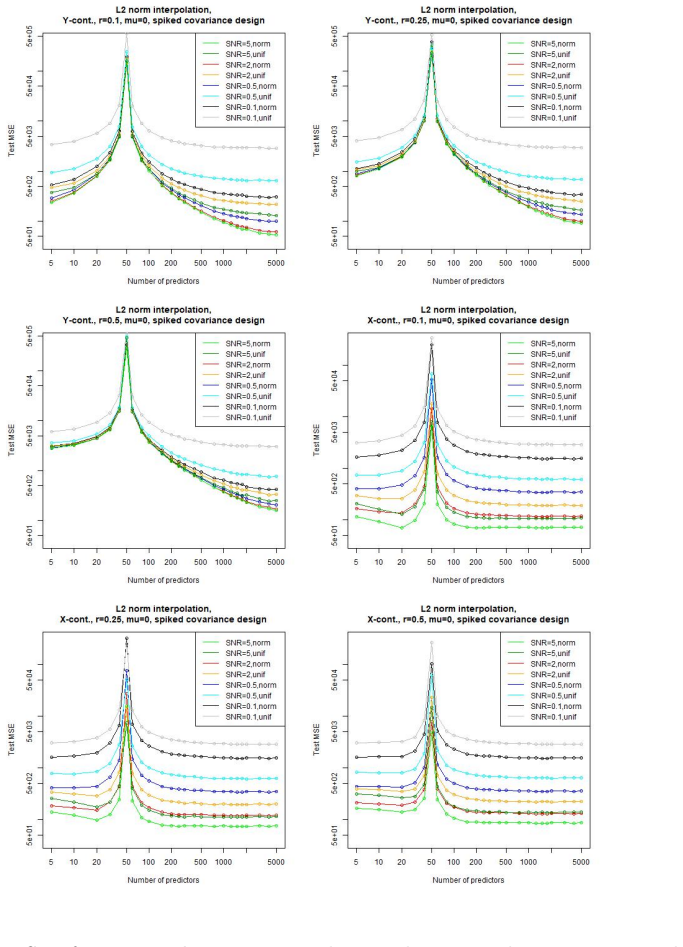
Figure 1. Figure 1: Test MSE of minimum l2-norm interpolation when trained on clean training data. In [PITH_FULL_IMAGE:figures/full_fig_p009_1.png] view at source ↗
Figure 2
Figure 2. Figure 2: Test MSE of minimum l2-norm interpolation when trained on contaminated training data. 10 [PITH_FULL_IMAGE:figures/full_fig_p010_2.png] view at source ↗
Figure 3
Figure 3. Figure 3: Test MSE of Huber-loss interpolation when trained on clean training data. The main difference between the MSE curves in [PITH_FULL_IMAGE:figures/full_fig_p011_3.png] view at source ↗
Figure 4
Figure 4. Figure 4: Test MSE of Huber-loss interpolation when trained on contaminated training data. 12 [PITH_FULL_IMAGE:figures/full_fig_p012_4.png] view at source ↗
Figure 5
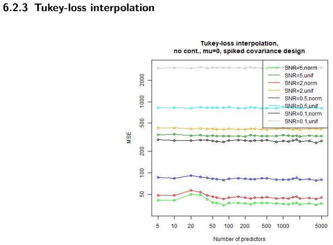
Figure 5. Figure 5: Test MSE of Tukey-loss interpolation when trained on clean training data. In [PITH_FULL_IMAGE:figures/full_fig_p013_5.png] view at source ↗
Figure 6
Figure 6. Figure 6: Test MSE of Tukey-loss interpolation when trained on contaminated training data. 14 [PITH_FULL_IMAGE:figures/full_fig_p014_6.png] view at source ↗
Figure 7
Figure 7. Figure 7: Test MSE of SLTS-based interpolation when trained on clean training data [PITH_FULL_IMAGE:figures/full_fig_p015_7.png] view at source ↗
Figure 8
Figure 8. Figure 8: Test MSE of SLTS when trained on clean training data. 15 [PITH_FULL_IMAGE:figures/full_fig_p015_8.png] view at source ↗
Figure 9
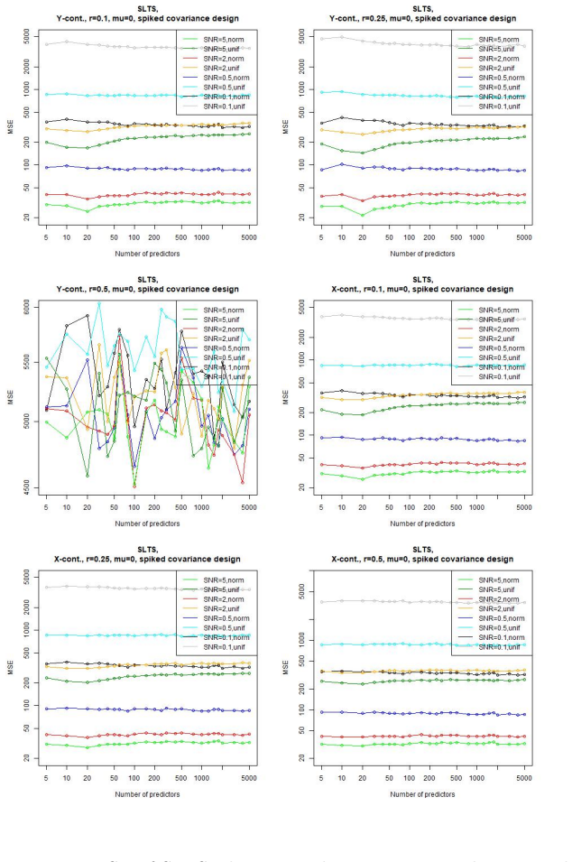
Figure 9. Figure 9: Test MSE of SLTS-based interpolation when trained on contaminated training data. In [PITH_FULL_IMAGE:figures/full_fig_p016_9.png] view at source ↗
Figure 10
Figure 10. Figure 10: Test MSE of SLTS when trained on contaminated training data. Standard SLTS results in similar MSE curves when trained on clean data as SLTS-based in￾terpolation, as it can be observed in [PITH_FULL_IMAGE:figures/full_fig_p017_10.png] view at source ↗
Figure 11
Figure 11. Figure 11: Test MSE of RRBoost-based interpolation when trained on clean training data [PITH_FULL_IMAGE:figures/full_fig_p018_11.png] view at source ↗
Figure 12
Figure 12. Figure 12: Test MSE of RRBoost when trained on clean training data. 18 [PITH_FULL_IMAGE:figures/full_fig_p018_12.png] view at source ↗
Figure 13
Figure 13. Figure 13: Test MSE of RRBoost-based interpolation when trained on contaminated training data. The MSE curves in [PITH_FULL_IMAGE:figures/full_fig_p019_13.png] view at source ↗
Figure 14
Figure 14. Figure 14: Test MSE of RRBoost when trained on contaminated training data. In contrast to RRBoost-based interpolation, the MSE curves slightly increase for growing p in [PITH_FULL_IMAGE:figures/full_fig_p020_14.png] view at source ↗
Figure 15
Figure 15. Figure 15: Test MSE of minimum l2-norm interpolation when trained on clean training data. 21 [PITH_FULL_IMAGE:figures/full_fig_p021_15.png] view at source ↗
Figure 16
Figure 16. Figure 16: Test MSE of minimum l2-norm interpolation when trained on contaminated training data. 22 [PITH_FULL_IMAGE:figures/full_fig_p022_16.png] view at source ↗
Figure 17
Figure 17. Figure 17: Test MSE of Huber-loss interpolation when trained on clean training data. 23 [PITH_FULL_IMAGE:figures/full_fig_p023_17.png] view at source ↗
Figure 18
Figure 18. Figure 18: Test MSE of Huber-loss interpolation when trained on contaminated training data. 24 [PITH_FULL_IMAGE:figures/full_fig_p024_18.png] view at source ↗
Figure 19
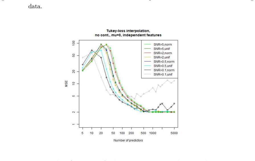
Figure 19. Figure 19: Test MSE of Tukey-loss interpolation when trained on clean training data. 25 [PITH_FULL_IMAGE:figures/full_fig_p025_19.png] view at source ↗
Figure 20
Figure 20. Figure 20: Test MSE of Tukey-loss interpolation when trained on contaminated training data. 26 [PITH_FULL_IMAGE:figures/full_fig_p026_20.png] view at source ↗
Figure 21
Figure 21. Figure 21: Test MSE of SLTS-based interpolation when trained on clean training data [PITH_FULL_IMAGE:figures/full_fig_p027_21.png] view at source ↗
Figure 22
Figure 22. Figure 22: Test MSE of SLTS when trained on clean training data. 27 [PITH_FULL_IMAGE:figures/full_fig_p027_22.png] view at source ↗
Figure 23
Figure 23. Figure 23: Test MSE of SLTS-based interpolation when trained on contaminated training data. 28 [PITH_FULL_IMAGE:figures/full_fig_p028_23.png] view at source ↗
Figure 24
Figure 24. Figure 24: Test MSE of SLTS when trained on contaminated training data. 29 [PITH_FULL_IMAGE:figures/full_fig_p029_24.png] view at source ↗
Figure 25
Figure 25. Figure 25: Test MSE of RRBoost-based interpolation when trained on clean training data [PITH_FULL_IMAGE:figures/full_fig_p030_25.png] view at source ↗
Figure 26
Figure 26. Figure 26: Test MSE of RRBoost when trained on clean training data. 30 [PITH_FULL_IMAGE:figures/full_fig_p030_26.png] view at source ↗
Figure 27
Figure 27. Figure 27: Test MSE of RRBoost-based interpolation when trained on contaminated training data. 31 [PITH_FULL_IMAGE:figures/full_fig_p031_27.png] view at source ↗
Figure 28
Figure 28. Figure 28: Test MSE of RRBoost when trained on contaminated training data. The curves in [PITH_FULL_IMAGE:figures/full_fig_p032_28.png] view at source ↗
Figure 29
Figure 29. Figure 29: Test MSE of minimum l2-norm interpolation when trained on clean training data with µ = 5. In contrast to the case µ = 0, the MSE curves for Y -contamination remain around the MSE values for small p after the peak. In the case of X-contamination and clean training data, the curves resemble those from the case µ = 0, with the difference that the MSE values are higher, as depicted in [PITH_FULL_IMAGE:figure… view at source ↗
Figure 30
Figure 30. Figure 30: Test MSE of minimum l2-norm interpolation when trained on contaminated training data with µ = 5. 34 [PITH_FULL_IMAGE:figures/full_fig_p034_30.png] view at source ↗
Figure 31
Figure 31. Figure 31: Test MSE of Huber-loss interpolation when trained on clean training data. As one can observe in [PITH_FULL_IMAGE:figures/full_fig_p035_31.png] view at source ↗
Figure 32
Figure 32. Figure 32: Test MSE of Huber-loss interpolation when trained on contaminated training data. 36 [PITH_FULL_IMAGE:figures/full_fig_p036_32.png] view at source ↗
Figure 33
Figure 33. Figure 33: Test MSE of SLTS-based interpolation when trained on clean training data [PITH_FULL_IMAGE:figures/full_fig_p037_33.png] view at source ↗
Figure 34
Figure 34. Figure 34: Test MSE of SLTS when trained on clean training data. 37 [PITH_FULL_IMAGE:figures/full_fig_p037_34.png] view at source ↗
Figure 35
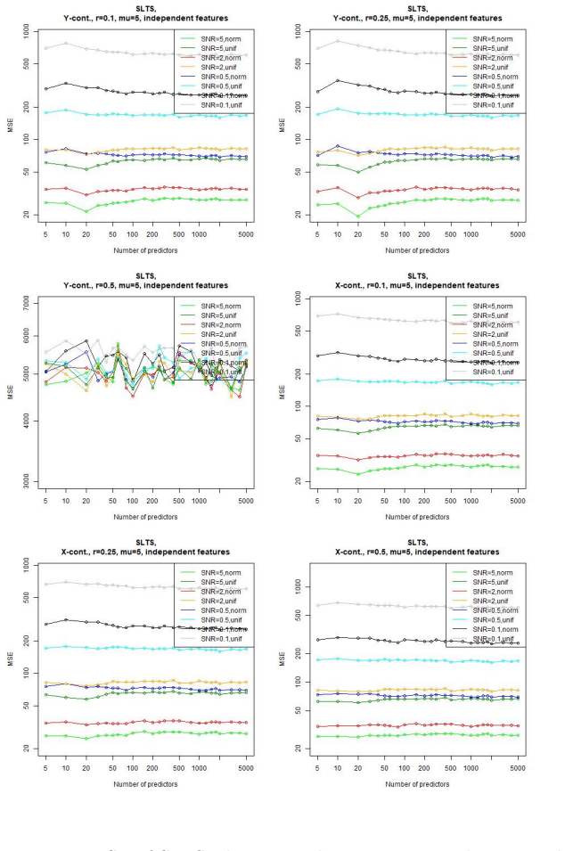
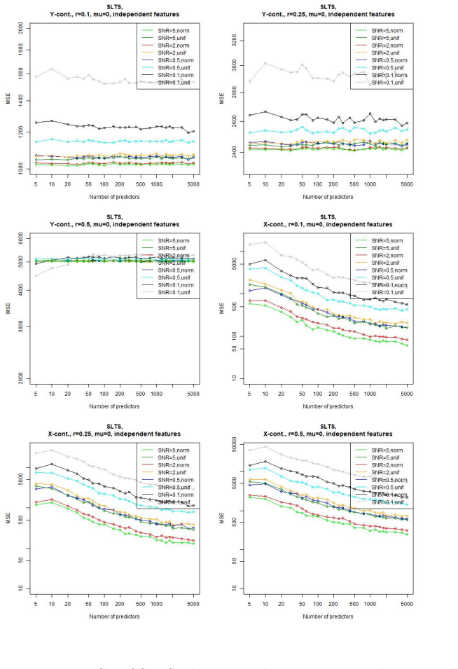
Figure 35. Figure 35: Test MSE of SLTS-based interpolation when trained on contaminated training data. 38 [PITH_FULL_IMAGE:figures/full_fig_p038_35.png] view at source ↗
Figure 36
Figure 36. Figure 36: Test MSE of SLTS when trained on contaminated training data. The MSE curves depicted in [PITH_FULL_IMAGE:figures/full_fig_p039_36.png] view at source ↗
Figure 37
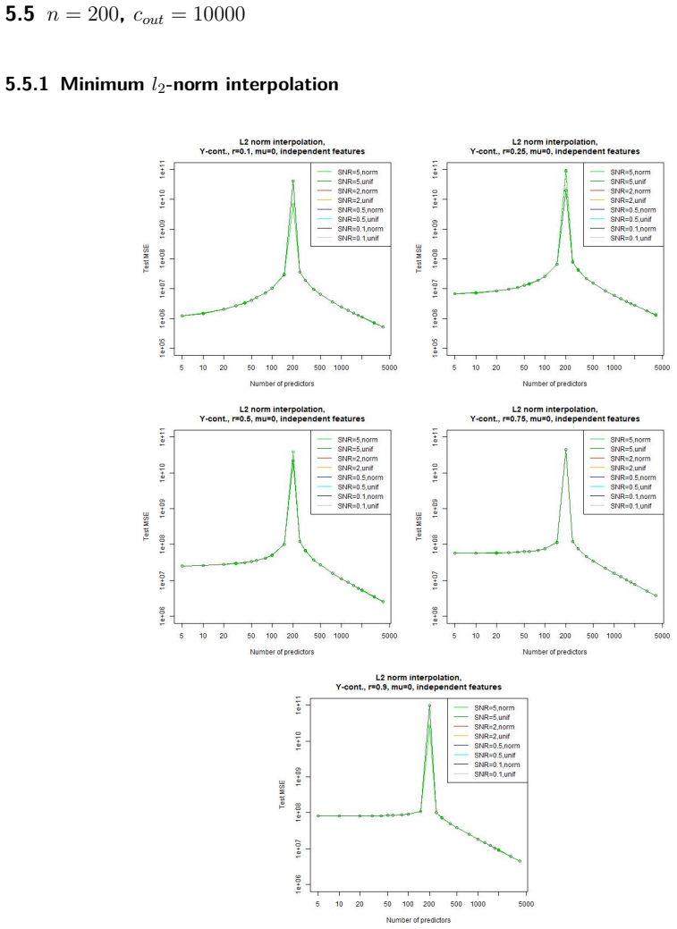
Figure 37. Figure 37: Test MSE of minimum l2-norm interpolation when trained on Y -contaminated train￾ing data. In contrast to the case n = 50 in [PITH_FULL_IMAGE:figures/full_fig_p040_37.png] view at source ↗
Figure 38
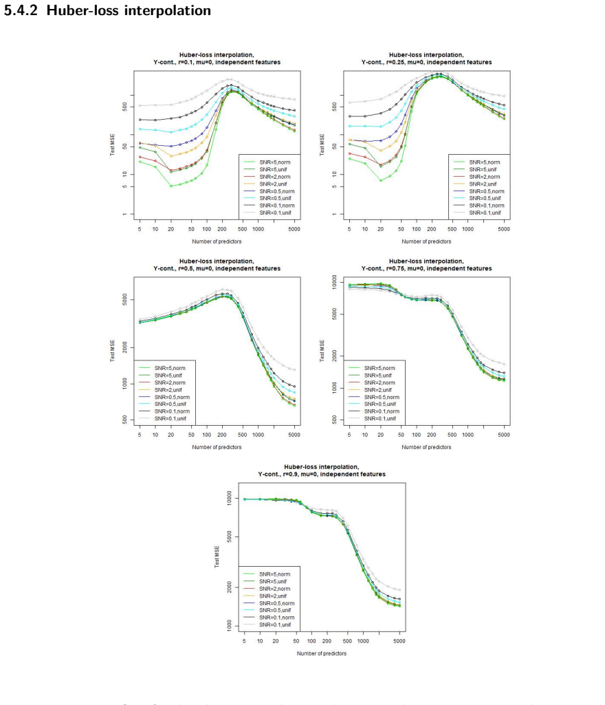
Figure 38. Figure 38: Test MSE of Huber-loss interpolation when trained on Y -contaminated training data. The MSE curves in [PITH_FULL_IMAGE:figures/full_fig_p041_38.png] view at source ↗
Figure 39
Figure 39. Figure 39: Test MSE of minimum l2-norm interpolation when trained on Y -contaminated train￾ing data. The MSE curves in [PITH_FULL_IMAGE:figures/full_fig_p042_39.png] view at source ↗
Figure 40
Figure 40. Figure 40: Test MSE of Huber-loss interpolation when trained on Y -contaminated training data. For r ∈ {0.1, 0.25}, the MSE curves in [PITH_FULL_IMAGE:figures/full_fig_p043_40.png] view at source ↗
Figure 41
Figure 41. Figure 41: Training MSE of minimum l2-norm interpolation when trained on clean training data. By interpolation, the training error vanishes once p > n, as depicted in [PITH_FULL_IMAGE:figures/full_fig_p044_41.png] view at source ↗
Figure 42
Figure 42. Figure 42: Training MSE of minimum l2-norm interpolation when trained on contaminated train￾ing data. 45 [PITH_FULL_IMAGE:figures/full_fig_p045_42.png] view at source ↗
Figure 43
Figure 43. Figure 43: Training MSE of Huber-loss interpolation when trained on clean training data. The training error curves in [PITH_FULL_IMAGE:figures/full_fig_p046_43.png] view at source ↗
Figure 44
Figure 44. Figure 44: Training MSE of Huber-loss interpolation when trained on contaminated training data. 47 [PITH_FULL_IMAGE:figures/full_fig_p047_44.png] view at source ↗
Figure 45
Figure 45. Figure 45: Training MSE of Tukey-loss interpolation when trained on clean training data. The training MSE for Tukey-loss interpolation, as depicted in [PITH_FULL_IMAGE:figures/full_fig_p048_45.png] view at source ↗
Figure 46
Figure 46. Figure 46: Training MSE of Tukey-loss interpolation when trained on contaminated training data. 49 [PITH_FULL_IMAGE:figures/full_fig_p049_46.png] view at source ↗
Figure 47
Figure 47. Figure 47: Training MSE of SLTS-based interpolation when trained on clean training data [PITH_FULL_IMAGE:figures/full_fig_p050_47.png] view at source ↗
Figure 48
Figure 48. Figure 48: Training MSE of SLTS when trained on clean training data. 50 [PITH_FULL_IMAGE:figures/full_fig_p050_48.png] view at source ↗
Figure 49
Figure 49. Figure 49: Training MSE of SLTS-based interpolation when trained on contaminated training data. 51 [PITH_FULL_IMAGE:figures/full_fig_p051_49.png] view at source ↗
Figure 50
Figure 50. Figure 50: Training MSE of SLTS when trained on contaminated training data. Neither SLTS-based interpolation nor SLTS leads to a vanishing training loss, since the model is trained only on a clean subset. As for the case of clean training data, as depicted in [PITH_FULL_IMAGE:figures/full_fig_p052_50.png] view at source ↗
Figure 51
Figure 51. Figure 51: Training MSE of RRBoost-based interpolation when trained on clean training data [PITH_FULL_IMAGE:figures/full_fig_p053_51.png] view at source ↗
Figure 52
Figure 52. Figure 52: Training MSE of RRBoost when trained on clean training data. 53 [PITH_FULL_IMAGE:figures/full_fig_p053_52.png] view at source ↗
Figure 53
Figure 53. Figure 53: Training MSE of RRBoost-based interpolation when trained on contaminated train￾ing data. 54 [PITH_FULL_IMAGE:figures/full_fig_p054_53.png] view at source ↗
Figure 54
Figure 54. Figure 54: Training MSE of RRBoost when trained on contaminated training data. For RRBoost-based interpolation, [PITH_FULL_IMAGE:figures/full_fig_p055_54.png] view at source ↗
Figure 55
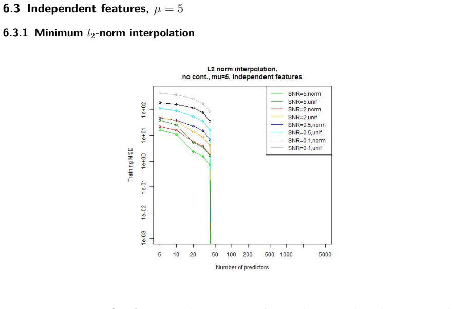
Figure 55. Figure 55: Training MSE of minimum l2-norm interpolation when trained on clean training data. 56 [PITH_FULL_IMAGE:figures/full_fig_p056_55.png] view at source ↗
Figure 56
Figure 56. Figure 56: Training MSE of minimum l2-norm interpolation when trained on contaminated train￾ing data. 57 [PITH_FULL_IMAGE:figures/full_fig_p057_56.png] view at source ↗
Figure 57
Figure 57. Figure 57: Training MSE of Huber-loss interpolation when trained on clean training data. 58 [PITH_FULL_IMAGE:figures/full_fig_p058_57.png] view at source ↗
Figure 58
Figure 58. Figure 58: Training MSE of Huber-loss interpolation when trained on contaminated training data. 59 [PITH_FULL_IMAGE:figures/full_fig_p059_58.png] view at source ↗
Figure 59
Figure 59. Figure 59: Training MSE of Tukey-loss interpolation when trained on clean training data. 60 [PITH_FULL_IMAGE:figures/full_fig_p060_59.png] view at source ↗
Figure 60
Figure 60. Figure 60: Training MSE of Tukey-loss interpolation when trained on contaminated training data. 61 [PITH_FULL_IMAGE:figures/full_fig_p061_60.png] view at source ↗
Figure 61
Figure 61. Figure 61: Training MSE of SLTS-based interpolation when trained on clean training data [PITH_FULL_IMAGE:figures/full_fig_p062_61.png] view at source ↗
Figure 62
Figure 62. Figure 62: Training MSE of SLTS when trained on clean training data. 62 [PITH_FULL_IMAGE:figures/full_fig_p062_62.png] view at source ↗
Figure 63
Figure 63. Figure 63: Training MSE of SLTS-based interpolation when trained on contaminated training data. 63 [PITH_FULL_IMAGE:figures/full_fig_p063_63.png] view at source ↗
Figure 64
Figure 64. Figure 64: Training MSE of SLTS when trained on contaminated training data. 64 [PITH_FULL_IMAGE:figures/full_fig_p064_64.png] view at source ↗
Figure 65
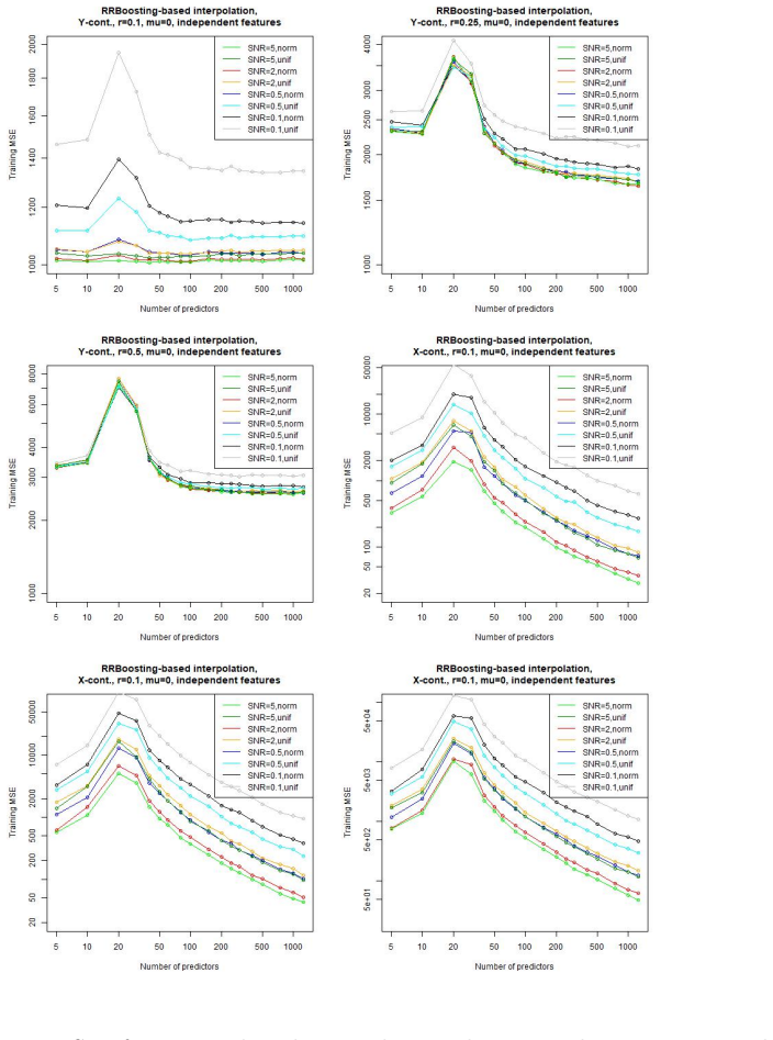
Figure 65. Figure 65: Training MSE of RRBoost-based interpolation when trained on clean training data [PITH_FULL_IMAGE:figures/full_fig_p065_65.png] view at source ↗
Figure 66
Figure 66. Figure 66: Training MSE of RRBoost-based interpolation when trained on clean training data. 65 [PITH_FULL_IMAGE:figures/full_fig_p065_66.png] view at source ↗
Figure 67
Figure 67. Figure 67: Training MSE of RRBoosting when trained on contaminated training data. 66 [PITH_FULL_IMAGE:figures/full_fig_p066_67.png] view at source ↗
Figure 68
Figure 68. Figure 68: Training MSE of RRBoosting when trained on contaminated training data. It can be observed in [PITH_FULL_IMAGE:figures/full_fig_p067_68.png] view at source ↗
Figure 69
Figure 69. Figure 69: Training MSE of minimum l2-norm interpolation when trained on clean training data. 68 [PITH_FULL_IMAGE:figures/full_fig_p068_69.png] view at source ↗
Figure 70
Figure 70. Figure 70: Training MSE of minimum l2-norm interpolation when trained on contaminated train￾ing data. 69 [PITH_FULL_IMAGE:figures/full_fig_p069_70.png] view at source ↗
Figure 71
Figure 71. Figure 71: Training MSE of Huber-loss interpolation when trained on clean training data. 70 [PITH_FULL_IMAGE:figures/full_fig_p070_71.png] view at source ↗
Figure 72
Figure 72. Figure 72: Training MSE of Huber-loss interpolation when trained on contaminated training data. 71 [PITH_FULL_IMAGE:figures/full_fig_p071_72.png] view at source ↗
Figure 73
Figure 73. Figure 73: Training MSE of SLTS-based interpolation when trained on clean training data [PITH_FULL_IMAGE:figures/full_fig_p072_73.png] view at source ↗
Figure 74
Figure 74. Figure 74: Training MSE of SLTS when trained on clean training data. 72 [PITH_FULL_IMAGE:figures/full_fig_p072_74.png] view at source ↗
Figure 75
Figure 75. Figure 75: Training MSE of SLTS-based interpolation when trained on contaminated training data. 73 [PITH_FULL_IMAGE:figures/full_fig_p073_75.png] view at source ↗
Figure 76
Figure 76. Figure 76: Training MSE of SLTS when trained on contaminated training data. It can be observed in [PITH_FULL_IMAGE:figures/full_fig_p074_76.png] view at source ↗
Figure 77
Figure 77. Figure 77: Training MSE of minimum l2-norm interpolation when trained on Y -contaminated training data. The training MSE vanishes at p = n, as expected (it is an issue of the plot function in R that it seems that the MSE vanishes earlier in [PITH_FULL_IMAGE:figures/full_fig_p075_77.png] view at source ↗
Figure 78
Figure 78. Figure 78: Training MSE of Huber-loss interpolation when trained on Y -contaminated training data. It already has been observed in [PITH_FULL_IMAGE:figures/full_fig_p076_78.png] view at source ↗
Figure 79
Figure 79. Figure 79: Training MSE of minimum l2-norm interpolation when trained on Y -contaminated training data. The training MSE curves in [PITH_FULL_IMAGE:figures/full_fig_p077_79.png] view at source ↗
Figure 80
Figure 80. Figure 80: Training MSE of Huber-loss interpolation when trained on Y -contaminated training data. The training MSE curves in [PITH_FULL_IMAGE:figures/full_fig_p078_80.png] view at source ↗
Figure 81
Figure 81. Figure 81: Differences ||βˆ − β||1/n for the estimated coefficient vector βˆ of minimum l2-norm interpolation when trained on clean training data and the true coefficient vector β. 79 [PITH_FULL_IMAGE:figures/full_fig_p079_81.png] view at source ↗
Figure 82
Figure 82. Figure 82: Differences ||βˆ − β||1/n for the estimated coefficient vector βˆ of minimum l2-norm interpolation when trained on contaminated training data and the true coefficient vector β. One can observe in [PITH_FULL_IMAGE:figures/full_fig_p080_82.png] view at source ↗
Figure 83
Figure 83. Figure 83: Differences ||βˆ − β||1/n for the estimated coefficient vector βˆ of Huber-loss interpo￾lation when trained on clean training data and the true coefficient vector β. 81 [PITH_FULL_IMAGE:figures/full_fig_p081_83.png] view at source ↗
Figure 84
Figure 84. Figure 84: Differences ||βˆ − β||1/n for the estimated coefficient vector βˆ of Huber-loss interpo￾lation when trained on contaminated training data and the true coefficient vector β. The curves in [PITH_FULL_IMAGE:figures/full_fig_p082_84.png] view at source ↗
Figure 85
Figure 85. Figure 85: Differences ||βˆ − β||1/n for the estimated coefficient vector βˆ of Tukey-loss interpo￾lation when trained on clean training data and the true coefficient vector β. 83 [PITH_FULL_IMAGE:figures/full_fig_p083_85.png] view at source ↗
Figure 86
Figure 86. Figure 86: Differences ||βˆ − β||1/n for the estimated coefficient vector βˆ of Tukey-loss interpo￾lation when trained on contaminated training data and the true coefficient vector β [PITH_FULL_IMAGE:figures/full_fig_p084_86.png] view at source ↗
Figure 87
Figure 87. Figure 87: Differences ||βˆ − β||1/n for the estimated coefficient vector βˆ of SLTS-based interpo￾lation when trained on clean training data and the true coefficient vector β [PITH_FULL_IMAGE:figures/full_fig_p085_87.png] view at source ↗
Figure 88
Figure 88. Figure 88: Differences ||βˆ − β||1/n for the estimated coefficient vector βˆ of SLTS when trained on clean training data and the true coefficient vector β. 85 [PITH_FULL_IMAGE:figures/full_fig_p085_88.png] view at source ↗
Figure 89
Figure 89. Figure 89: Differences ||βˆ − β||1/n for the estimated coefficient vector βˆ of SLTS-based inter￾polation when trained on contaminated training data and the true coefficient vector β. 86 [PITH_FULL_IMAGE:figures/full_fig_p086_89.png] view at source ↗
Figure 90
Figure 90. Figure 90: Differences ||βˆ − β||1/n for the estimated coefficient vector βˆ of SLTS when trained on contaminated training data and the true coefficient vector β [PITH_FULL_IMAGE:figures/full_fig_p087_90.png] view at source ↗
Figure 91
Figure 91. Figure 91: Differences ||βˆ − β||1/n for the estimated coefficient vector βˆ of RRBoosting-based interpolation when trained on clean training data and the true coefficient vector β. 88 [PITH_FULL_IMAGE:figures/full_fig_p088_91.png] view at source ↗
Figure 92
Figure 92. Figure 92: Differences ||βˆ − β||1/n for the estimated coefficient vector βˆ of RRBoosting-based interpolation when trained on contaminated training data and the true coefficient vector β [PITH_FULL_IMAGE:figures/full_fig_p089_92.png] view at source ↗
Figure 93
Figure 93. Figure 93: Differences ||βˆ − β||1/n for the estimated coefficient vector βˆ of minimum l2-norm interpolation when trained on clean training data and the true coefficient vector β. 90 [PITH_FULL_IMAGE:figures/full_fig_p090_93.png] view at source ↗
Figure 94
Figure 94. Figure 94: Differences ||βˆ − β||1/n for the estimated coefficient vector βˆ of minimum l2-norm interpolation when trained on contaminated training data and the true coefficient vector β. 91 [PITH_FULL_IMAGE:figures/full_fig_p091_94.png] view at source ↗
Figure 95
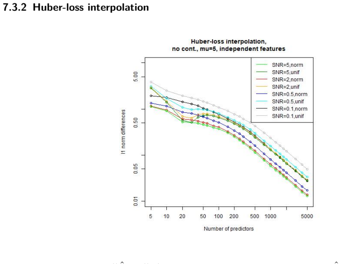
Figure 95. Figure 95: Differences ||βˆ− β||1/n for the estimated coefficient vector βˆ of Huber-norm interpo￾lation when trained on clean training data and the true coefficient vector β. 92 [PITH_FULL_IMAGE:figures/full_fig_p092_95.png] view at source ↗
Figure 96
Figure 96. Figure 96: Differences ||βˆ − β||1/n for the estimated coefficient vector βˆ of Huber-norm inter￾polation when trained on contaminated training data and the true coefficient vector β. 93 [PITH_FULL_IMAGE:figures/full_fig_p093_96.png] view at source ↗
Figure 97
Figure 97. Figure 97: Differences ||βˆ− β||1/n for the estimated coefficient vector βˆ of Tukey-norm interpo￾lation when trained on clean training data and the true coefficient vector β. 94 [PITH_FULL_IMAGE:figures/full_fig_p094_97.png] view at source ↗
Figure 98
Figure 98. Figure 98: Differences ||βˆ − β||1/n for the estimated coefficient vector βˆ of Tukey-norm inter￾polation when trained on contaminated training data and the true coefficient vector β. 95 [PITH_FULL_IMAGE:figures/full_fig_p095_98.png] view at source ↗
Figure 99
Figure 99. Figure 99: Differences ||βˆ − β||1/n for the estimated coefficient vector βˆ of SLTS-based interpo￾lation when trained on clean training data and the true coefficient vector β [PITH_FULL_IMAGE:figures/full_fig_p096_99.png] view at source ↗
Figure 100
Figure 100. Figure 100: Differences ||βˆ − β||1/n for the estimated coefficient vector βˆ of SLTS when trained on clean training data and the true coefficient vector β. 96 [PITH_FULL_IMAGE:figures/full_fig_p096_100.png] view at source ↗
Figure 101
Figure 101. Figure 101: Differences ||βˆ − β||1/n for the estimated coefficient vector βˆ of SLTS-based inter￾polation when trained on contaminated training data and the true coefficient vector β. 97 [PITH_FULL_IMAGE:figures/full_fig_p097_101.png] view at source ↗
Figure 102
Figure 102. Figure 102: Differences ||βˆ − β||1/n for the estimated coefficient vector βˆ of SLTS when trained on contaminated training data and the true coefficient vector β. 98 [PITH_FULL_IMAGE:figures/full_fig_p098_102.png] view at source ↗
Figure 103
Figure 103. Figure 103: Differences ||βˆ − β||1/n for the estimated coefficient vector βˆ of RRBoosting-based interpolation when trained on clean training data and the true coefficient vector β. 99 [PITH_FULL_IMAGE:figures/full_fig_p099_103.png] view at source ↗
Figure 104
Figure 104. Figure 104: Differences ||βˆ − β||1/n for the estimated coefficient vector βˆ of RRBoosting-based interpolation when trained on contaminated training data and the true coefficient vector β. As one can observe in [PITH_FULL_IMAGE:figures/full_fig_p100_104.png] view at source ↗
Figure 105
Figure 105. Figure 105: Differences ||βˆ − β||1/n for the estimated coefficient vector βˆ of minimum l2-norm interpolation when trained on clean training data and the true coefficient vector β. 101 [PITH_FULL_IMAGE:figures/full_fig_p101_105.png] view at source ↗
Figure 106
Figure 106. Figure 106: Differences ||βˆ − β||1/n for the estimated coefficient vector βˆ of minimum l2-norm interpolation when trained on contaminated training data and the true coefficient vector β. 102 [PITH_FULL_IMAGE:figures/full_fig_p102_106.png] view at source ↗
Figure 107
Figure 107. Figure 107: Differences ||βˆ − β||1/n for the estimated coefficient vector βˆ of Huber-loss interpo￾lation when trained on clean training data and the true coefficient vector β. 103 [PITH_FULL_IMAGE:figures/full_fig_p103_107.png] view at source ↗
Figure 108
Figure 108. Figure 108: Differences ||βˆ − β||1/n for the estimated coefficient vector βˆ of Huber-loss interpo￾lation when trained on contaminated training data and the true coefficient vector β. 104 [PITH_FULL_IMAGE:figures/full_fig_p104_108.png] view at source ↗
Figure 109
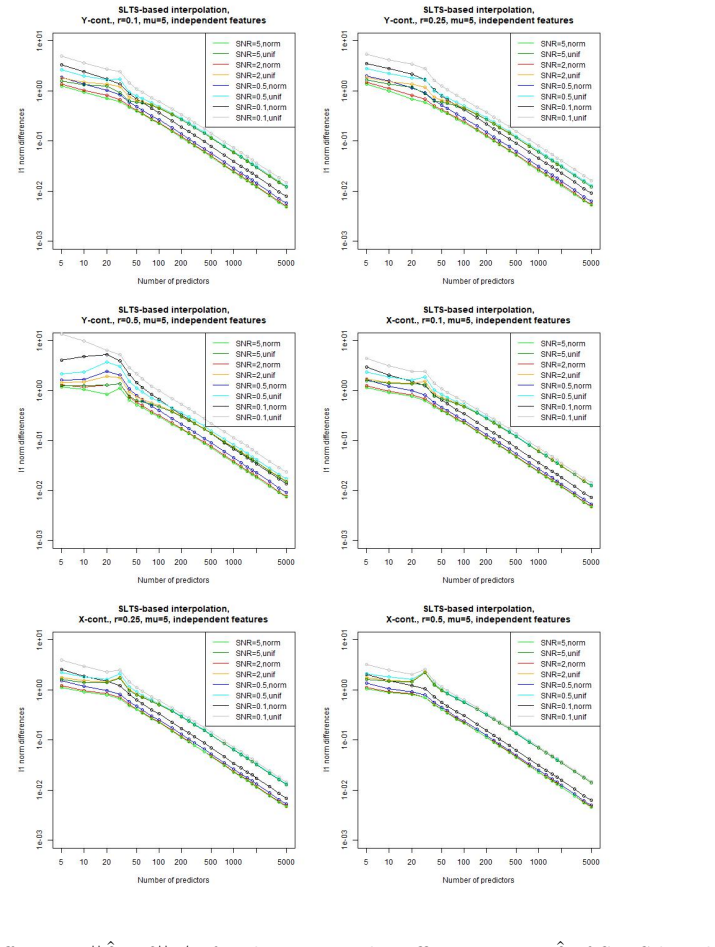
Figure 109. Figure 109: Differences ||βˆ − β||1/n for the estimated coefficient vector βˆ of SLTS-based inter￾polation when trained on clean training data and the true coefficient vector β [PITH_FULL_IMAGE:figures/full_fig_p105_109.png] view at source ↗
Figure 110
Figure 110. Figure 110: Differences ||βˆ − β||1/n for the estimated coefficient vector βˆ of SLTS when trained on clean training data and the true coefficient vector β. 105 [PITH_FULL_IMAGE:figures/full_fig_p105_110.png] view at source ↗
Figure 111
Figure 111. Figure 111: Differences ||βˆ − β||1/n for the estimated coefficient vector βˆ of SLTS-based inter￾polation when trained on contaminated training data and the true coefficient vector β. 106 [PITH_FULL_IMAGE:figures/full_fig_p106_111.png] view at source ↗
Figure 112
Figure 112. Figure 112: Differences ||βˆ − β||1/n for the estimated coefficient vector βˆ of SLTS when trained on contaminated training data and the true coefficient vector β. 107 [PITH_FULL_IMAGE:figures/full_fig_p107_112.png] view at source ↗
Figure 113
Figure 113. Figure 113: Differences ||βˆ − β||1/n for the estimated coefficient vector βˆ of RRBoosting-based interpolation when trained on clean training data and the true coefficient vector β. 108 [PITH_FULL_IMAGE:figures/full_fig_p108_113.png] view at source ↗
Figure 114
Figure 114. Figure 114: Differences ||βˆ − β||1/n for the estimated coefficient vector βˆ of RRBoosting-based interpolation when trained on contaminated training data and the true coefficient vector β [PITH_FULL_IMAGE:figures/full_fig_p109_114.png] view at source ↗
Figure 115
Figure 115. Figure 115: Differences ||βˆ − β||1/n for the estimated coefficient vector βˆ of minimum l2-norm interpolation when trained on Y -contaminated training data. 110 [PITH_FULL_IMAGE:figures/full_fig_p110_115.png] view at source ↗
Figure 116
Figure 116. Figure 116: Differences ||βˆ − β||1/n for the estimated coefficient vector βˆ of Huber-loss interpo￾lation when trained on Y -contaminated training data. The curves in [PITH_FULL_IMAGE:figures/full_fig_p111_116.png] view at source ↗
Figure 117
Figure 117. Figure 117: Differences ||βˆ − β||1/n for the estimated coefficient vector βˆ of minimum l2-norm interpolation when trained on Y -contaminated training data. The curves in [PITH_FULL_IMAGE:figures/full_fig_p112_117.png] view at source ↗
Figure 118
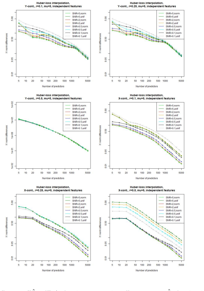
Figure 118. Figure 118: Differences ||βˆ − β||1/n for the estimated coefficient vector βˆ of Huber-loss interpo￾lation when trained on Y -contaminated training data. For r ∈ {0.1, 0.25}, the curves in [PITH_FULL_IMAGE:figures/full_fig_p113_118.png] view at source ↗
Figure 119
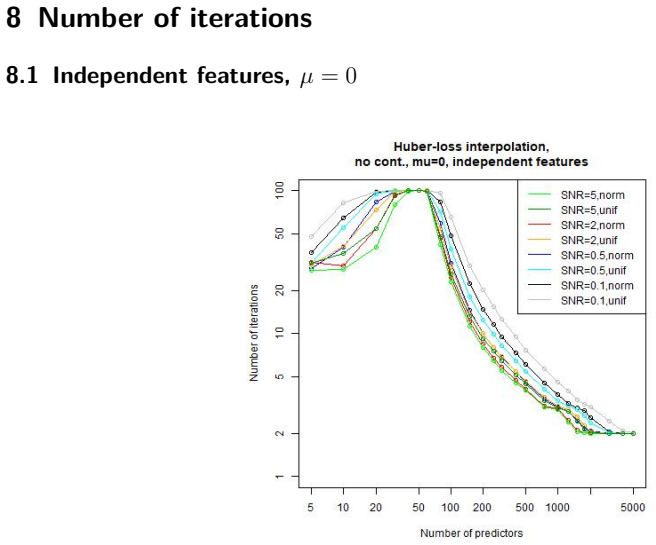
Figure 119. Figure 119: Mean number of iterations of Huber-loss interpolation when trained on clean training data [PITH_FULL_IMAGE:figures/full_fig_p114_119.png] view at source ↗
Figure 120
Figure 120. Figure 120: Mean number of iterations of Tukey-loss interpolation when trained on clean training data. 114 [PITH_FULL_IMAGE:figures/full_fig_p114_120.png] view at source ↗
Figure 121
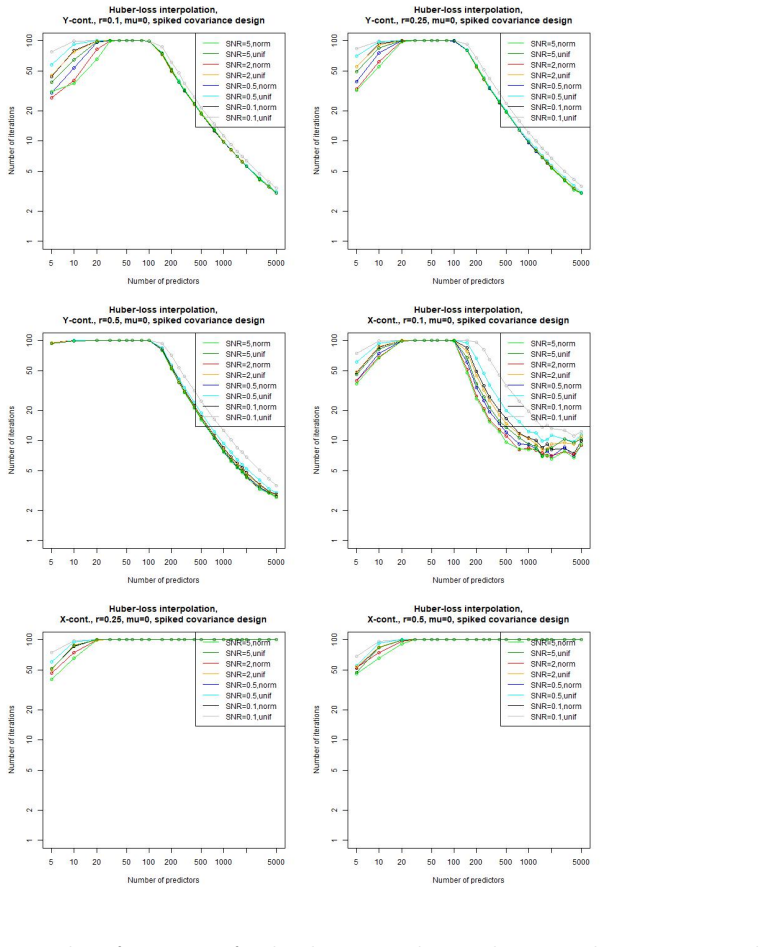
Figure 121. Figure 121: Mean number of iterations of Huber-loss interpolation when trained on contaminated training data. For Huber-loss based interpolation, as one can observe in [PITH_FULL_IMAGE:figures/full_fig_p115_121.png] view at source ↗
Figure 122
Figure 122. Figure 122: Mean number of iterations of Tukey-loss interpolation when trained on contaminated training data. For Tukey-based interpolation, [PITH_FULL_IMAGE:figures/full_fig_p116_122.png] view at source ↗
Figure 123
Figure 123. Figure 123: Mean number of iterations of Huber-loss interpolation when trained on clean training data. 117 [PITH_FULL_IMAGE:figures/full_fig_p117_123.png] view at source ↗
Figure 124
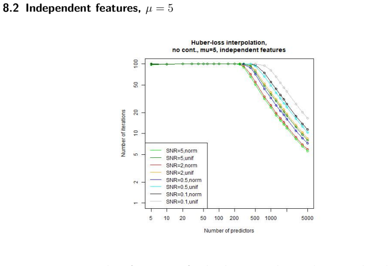
Figure 124. Figure 124: Mean number of iterations of Huber-loss interpolation when trained on contaminated training data. In contrast to the case µ = 0, the number of iterations stays much longer in the plateau and decreases for large p, as shown in [PITH_FULL_IMAGE:figures/full_fig_p118_124.png] view at source ↗
Figure 125
Figure 125. Figure 125: Mean number of iterations of Huber-loss interpolation when trained on clean training data [PITH_FULL_IMAGE:figures/full_fig_p119_125.png] view at source ↗
Figure 126
Figure 126. Figure 126: Mean number of iterations of Tukey-loss interpolation when trained on clean training data. 119 [PITH_FULL_IMAGE:figures/full_fig_p119_126.png] view at source ↗
Figure 127
Figure 127. Figure 127: Mean number of iterations of Huber-loss interpolation when trained on contaminated training data. 120 [PITH_FULL_IMAGE:figures/full_fig_p120_127.png] view at source ↗
Figure 128
Figure 128. Figure 128: Mean number of iterations of Tukey-loss interpolation when trained on contaminated training data. The curves, depicted in [PITH_FULL_IMAGE:figures/full_fig_p121_128.png] view at source ↗
Figure 129
Figure 129. Figure 129: Mean number of iterations of Huber-loss interpolation when trained on Y - contaminated training data. 122 [PITH_FULL_IMAGE:figures/full_fig_p122_129.png] view at source ↗
Figure 130
Figure 130. Figure 130: Mean number of iterations of Huber-loss interpolation when trained on Y - contaminated training data. 9 Discussion and conclusion 9.1 Discussion of the results The evaluation of the test MSEs in Sec. 5 reveals that the minimum l2-norm interpolator in￾deed shows the double descent behavior, as the MSE drops after the peak at p = n, provided a sufficiently high SNR (at least 2 in the experiments). Although… view at source ↗
read the original abstract

Overparametrized models can exhibit an excellent generalization performance, although they should be prone to overfitting according to classical statistical theory. The discovery of the "double descent", indicating that the generalization error decreases after a certain model complexity has been reached, opened a new line of research. Robust statistics considers statistical estimation on contaminated data, which, due to assumptions that do not hold on real data, let data points appear as outliers w.r.t. the assumed "ideal" distribution, potentially severely distorting any classical estimator. We address the question whether a double descent phenomenon can be observed in a linear regression setting with contaminated training data. We compare the performance of the highly non-robust least-squares interpolation estimator with several robust alternatives. It turns out that large overparametrization indeed allows for a double descent phenomenon, resulting in a very good generalization performance of the least-squares interpolator, surpassing that of the robust alternatives.
Editorial analysis
A structured set of objections, weighed in public.

Desk editor's note, referee report, simulated authors' rebuttal, and a circularity audit. Tearing a paper down is the easy half of reading it; the pith above is the substance, this is the friction.

Referee Report

2 major / 2 minor

Summary. The paper conducts a simulation study of linear regression under data contamination. It examines whether the least-squares interpolator exhibits double descent in test error as the overparameterization ratio grows and compares its generalization performance against several robust estimators, concluding that sufficiently large overparameterization yields a double-descent curve and that the interpolator ultimately outperforms the robust alternatives.

Significance. If the reported ordering proves stable under reasonable variations in contamination parameters, the result would indicate that classical interpolation can be surprisingly effective on contaminated data once models are heavily overparameterized. The work supplies concrete empirical evidence that double descent can appear in a robust-statistics setting and thereby supplies a useful data point for theoretical investigations of interpolation versus robustness.

major comments (2)
  1. [Simulation design] Simulation design (implicitly §3–4): the manuscript does not report the number of Monte Carlo repetitions, the precise outlier magnitude distribution, or error bars on the plotted curves. Because the central claim is that the LS interpolator surpasses robust estimators for large overparameterization, the absence of these quantities leaves open the possibility that the observed ordering is an artifact of a single draw or of a narrowly chosen contamination regime.
  2. [Results] Results section: the performance comparison is shown only for a fixed contamination fraction and a single outlier distribution. The claim that “large overparametrization indeed allows … surpassing that of the robust alternatives” therefore rests on an untested assumption that the relative ordering is insensitive to these simulation parameters; systematic sweeps or additional tables would be required to substantiate the generality of the reported superiority.
minor comments (2)
  1. [Notation] Notation for the overparameterization ratio and the contamination fraction should be defined once in a dedicated subsection and used consistently thereafter.
  2. [Figures] Figure captions should explicitly state the number of Monte Carlo runs and whether shaded regions represent standard errors or inter-quartile ranges.

Simulated Author's Rebuttal

2 responses · 0 unresolved

We thank the referee for the constructive comments, which help clarify the presentation of our simulation study. We address each major comment below and indicate the changes we will make.

read point-by-point responses
  1. Referee: [Simulation design] Simulation design (implicitly §3–4): the manuscript does not report the number of Monte Carlo repetitions, the precise outlier magnitude distribution, or error bars on the plotted curves. Because the central claim is that the LS interpolator surpasses robust estimators for large overparameterization, the absence of these quantities leaves open the possibility that the observed ordering is an artifact of a single draw or of a narrowly chosen contamination regime.

    Authors: We agree these details should have been stated explicitly for reproducibility. In the revised manuscript we will report the number of Monte Carlo repetitions, give the exact parameters of the outlier magnitude distribution, and add error bars (one standard deviation across repetitions) to the relevant figures. These additions will allow readers to assess the stability of the reported ordering. revision: yes

  2. Referee: [Results] Results section: the performance comparison is shown only for a fixed contamination fraction and a single outlier distribution. The claim that “large overparametrization indeed allows … surpassing that of the robust alternatives” therefore rests on an untested assumption that the relative ordering is insensitive to these simulation parameters; systematic sweeps or additional tables would be required to substantiate the generality of the reported superiority.

    Authors: The paper demonstrates that double descent and eventual superiority of the interpolator can occur under contamination for the chosen representative parameters; it does not claim this ordering holds for every possible contamination regime. We will revise the text to make the scope of the claims explicit and add a short discussion of sensitivity. We will also include one supplementary table showing results for a second contamination fraction to provide additional support without expanding the scope into a full parameter sweep. revision: partial

Circularity Check

0 steps flagged

No significant circularity in simulation-based analysis

full rationale

This is a simulation study that generates results by running forward Monte Carlo experiments on synthetic contaminated data under fixed contamination models and parameter choices. No equations are presented that define a target quantity in terms of a fitted parameter and then treat the simulation output as an independent prediction. There are no self-citations used to justify uniqueness theorems, no ansatzes smuggled via prior work, and no renaming of known results as new derivations. The performance ordering between least-squares interpolation and robust estimators is an observed outcome of the chosen simulation regime rather than a quantity forced by construction from the inputs. The paper is therefore self-contained against its own simulation benchmarks.

Axiom & Free-Parameter Ledger

2 free parameters · 1 axioms · 0 invented entities

The paper rests on simulation design choices rather than new theoretical axioms or invented entities; the main unverified elements are the representativeness of the contamination process and the choice of performance metrics.

free parameters (2)
  • contamination fraction and outlier distribution
    The proportion and statistical character of contaminated points are chosen by the authors to create the test regime.
  • overparameterization ratio
    The ratio of model dimension to sample size is varied across a range to trace the double-descent curve.
axioms (1)
  • domain assumption The simulated contamination model produces outliers whose effect on estimators is comparable to that encountered in real data.
    Invoked when the authors interpret the simulation results as relevant to robust statistics on contaminated data.

pith-pipeline@v0.9.0 · 5677 in / 1403 out tokens · 59628 ms · 2026-05-22T01:19:17.587973+00:00 · methodology

discussion (0)

Sign in with ORCID, Apple, or X to comment. Anyone can read and Pith papers without signing in.

Reference graph

Works this paper leans on

12 extracted references · 12 canonical work pages · 1 internal anchor

  1. [1]

    Y. Dar, V. Muthukumar, and R. G. Baraniuk. A farewell to the bias-variance trade- off? an overview of the theory of overparameterized machine learning.arXiv preprint arXiv:2109.02355,

  2. [2]

    Karhadkar, E

    K. Karhadkar, E. George, M. Murray, G. Montúfar, and D. Needell. Benign overfitting in leaky relu networks with moderate input dimension.arXiv preprint arXiv:2403.06903,

  3. [3]

    Kausik, K

    126 C. Kausik, K. Srivastava, and R. Sonthalia. Double descent and overfitting under noisy inputs and distribution shift for linear denoisers.arXiv preprint arXiv:2305.17297,

  4. [4]

    Koltchinskii

    V. Koltchinskii. Rademacher penalties and structural risk minimization.IEEE Transactions on Information Theory, 47(5):1902–1914,

  5. [5]

    arXiv preprint arXiv:1911.01544 , year=

    A. Montanari, F. Ruan, Y. Sohn, and J. Yan. The generalization error of max-margin linear classifiers: High-dimensional asymptotics in the overparametrized regime.arXiv preprint arXiv:1911.01544, 7,

  6. [6]

    Nakkiran, G

    P. Nakkiran, G. Kaplun, Y. Bansal, T. Yang, B. Barak, and I. Sutskever. Deep double descent: Where bigger models and more data hurt.Journal of Statistical Mechanics: Theory and Experiment, 2021(12):124003,

  7. [7]

    127 B. Neal, S. Mittal, A. Baratin, V. Tantia, M. Scicluna, S. Lacoste-Julien, and I. Mitliagkas. A modern take on the bias-variance tradeoff in neural networks.arXiv preprint arXiv:1810.08591,

  8. [8]

    Y. Qin, S. Li, Y. Li, and Y. Yu. Penalized maximum tangent likelihood estimation and robust variable selection.arXiv preprint arXiv:1708.05439,

  9. [9]

    Rahimi, T

    K. Rahimi, T. Tirer, and O. Lindenbaum. Multiple descents in unsupervised learning: The role of noise, domain shift and anomalies.arXiv preprint arXiv:2406.11703,

  10. [10]

    S. P. Singh, A. Lucchi, T. Hofmann, and B. Schölkopf. Phenomenology of double descent in finite-width neural networks.arXiv preprint arXiv:2203.07337,

  11. [11]

    Benign overfitting in rid ge regression

    A. Tsigler and P. L. Bartlett. Benign overfitting in ridge regression.arXiv preprint arXiv:2009.14286,

  12. [12]

    T. Werner. Robust statistics meets elicitability: When fair model validation breaks down.arXiv preprint arXiv:2405.09943,