Charting causal set configuration space with graph observables
Pith reviewed 2026-06-29 15:24 UTC · model grok-4.3
The pith
Three graph observables distinguish nine classes of causal sets by their low internal fluctuations.
A machine-rendered reading of the paper's core claim, the machinery that carries it, and where it could break.
Core claim
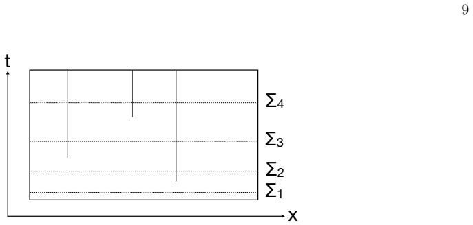
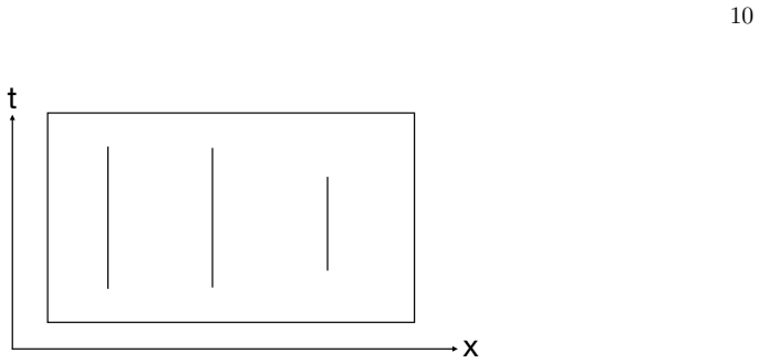
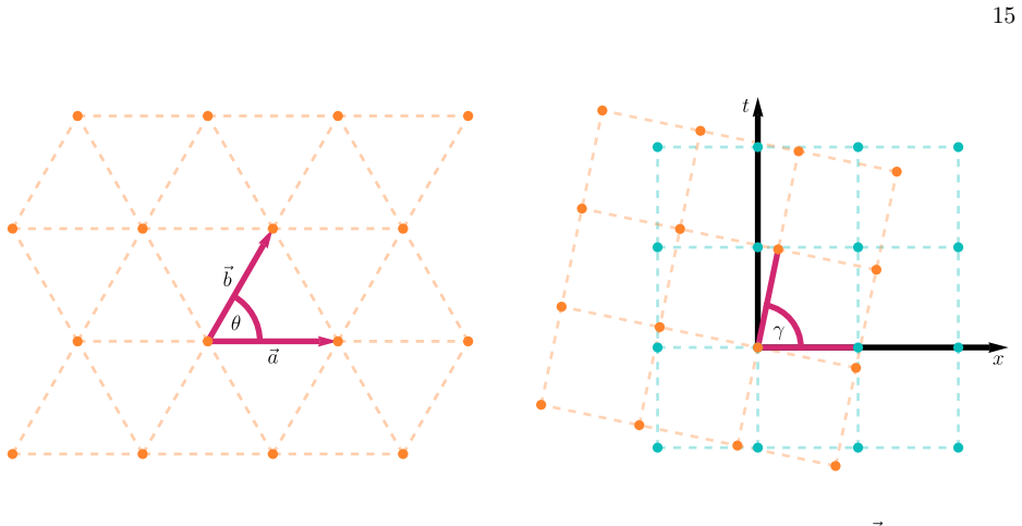
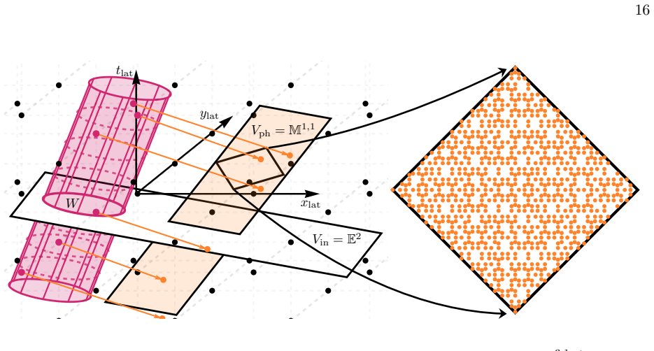
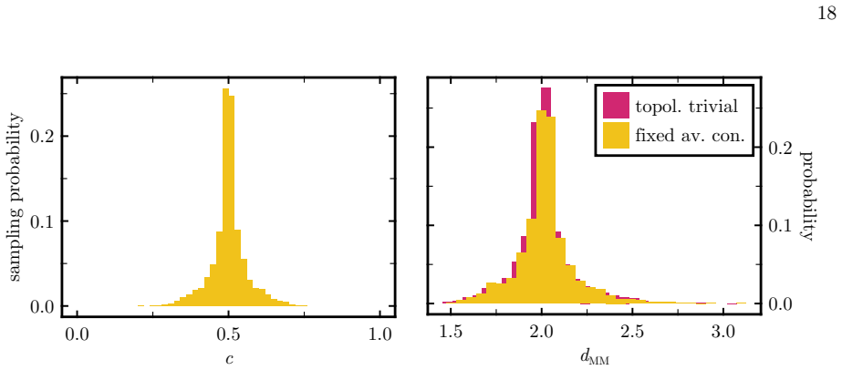
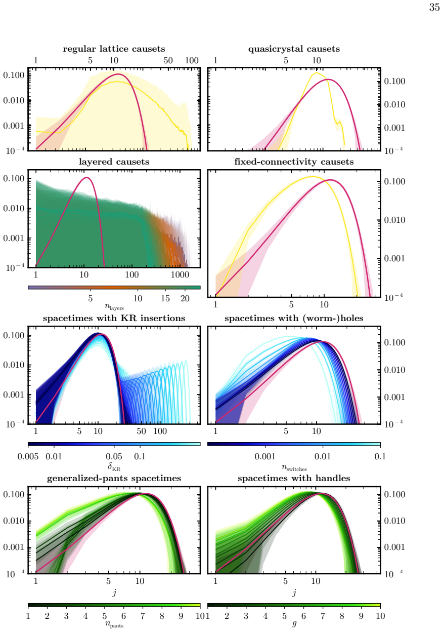
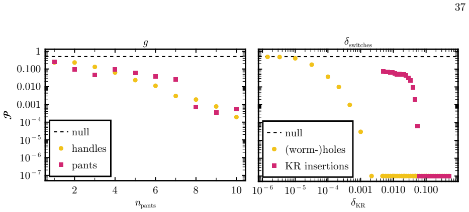
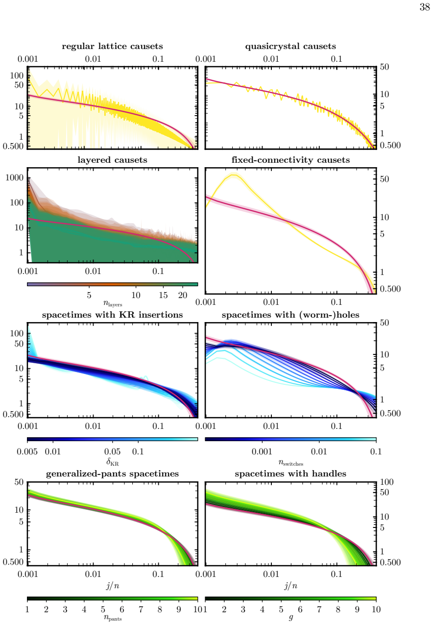
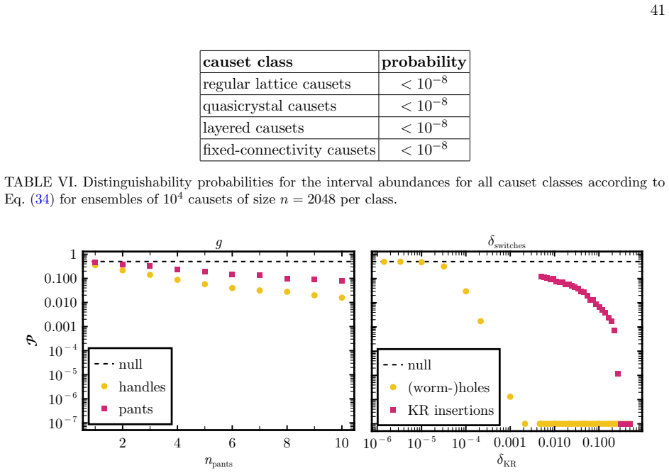
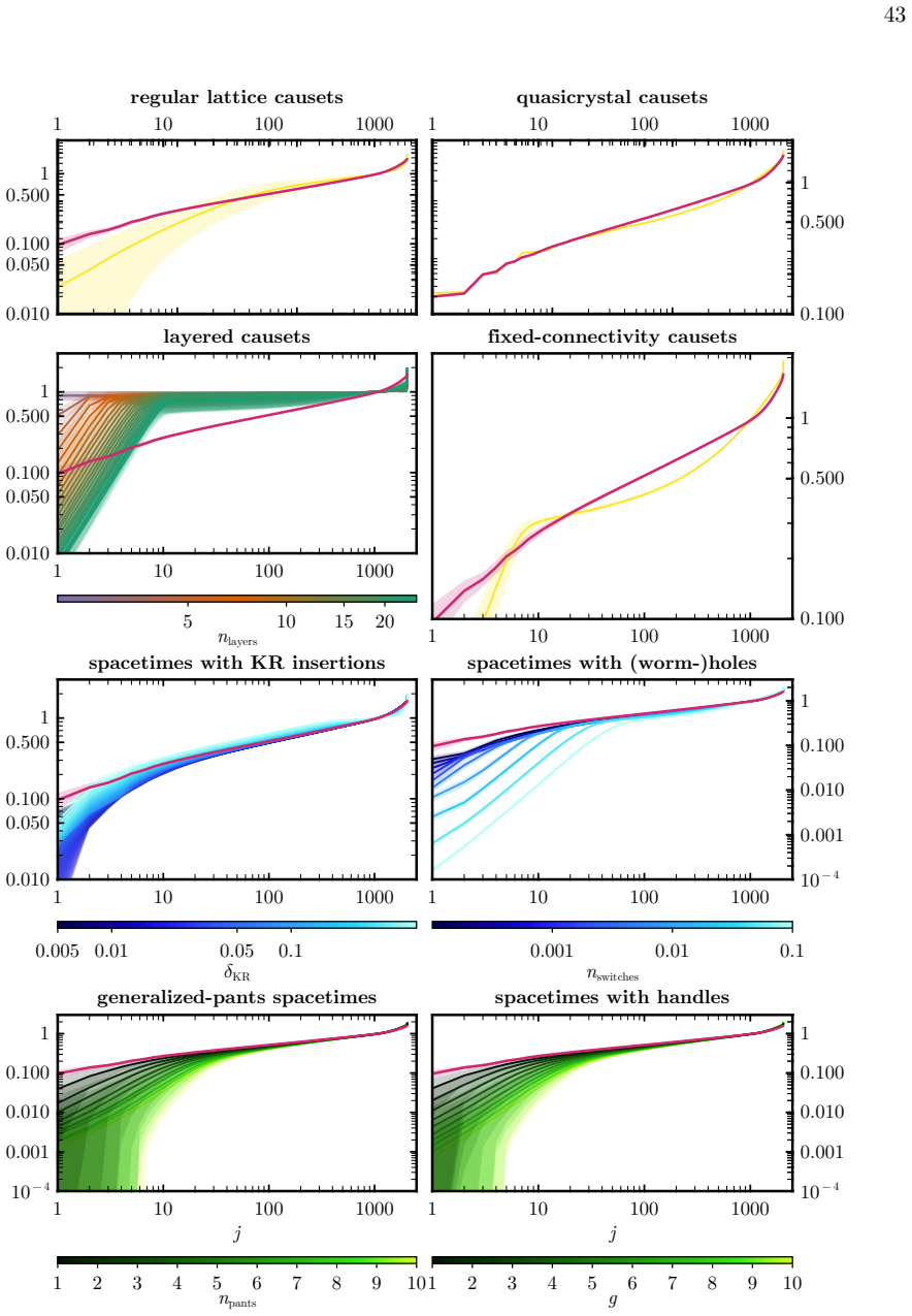
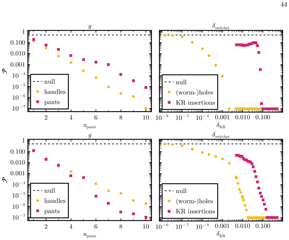
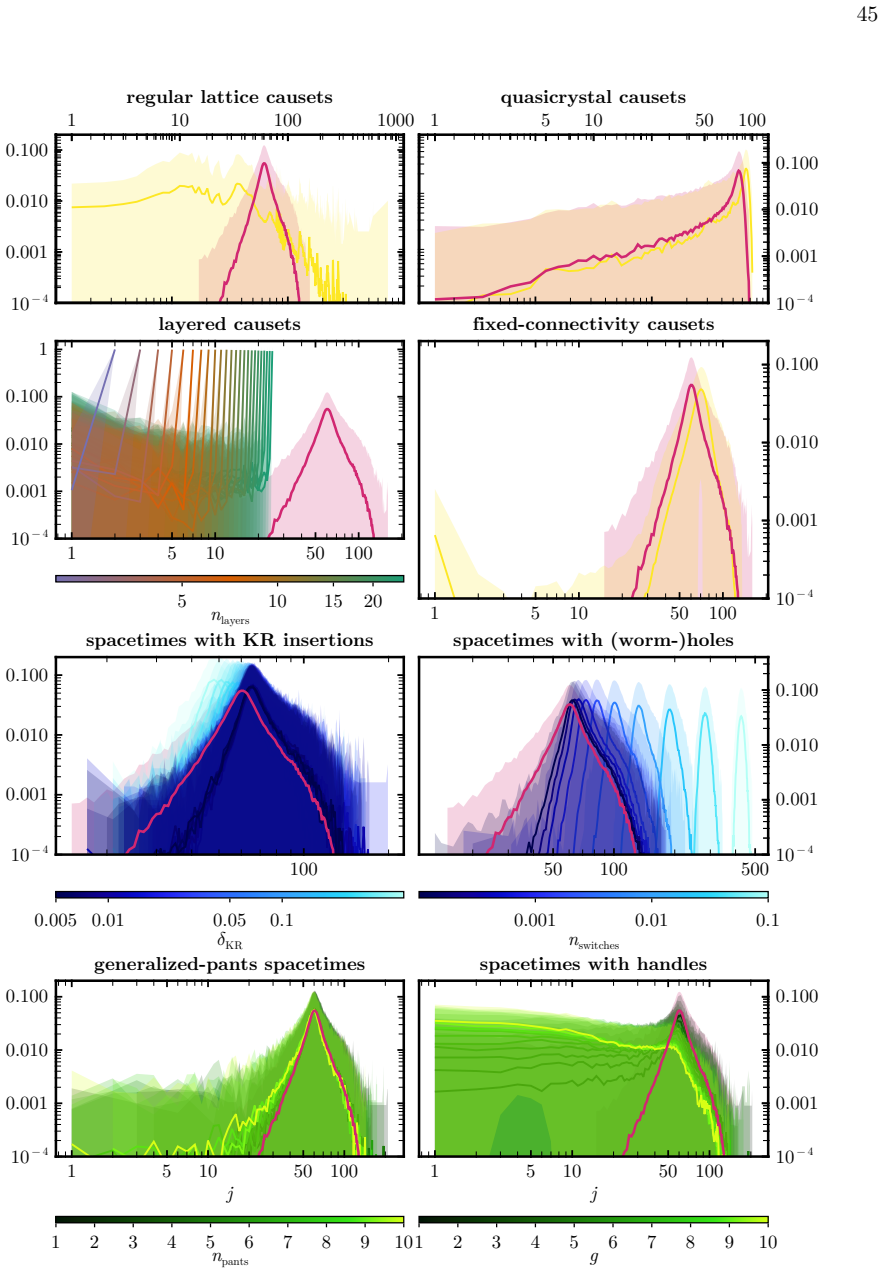
The paper establishes that the link degree distribution, the eigenvalues of the graph Laplacian of the symmetrized Hasse diagram, and the abundance of causal intervals can distinguish between nine classes of causal sets. These classes include manifoldlike sets with inhomogeneous Ricci curvature (both topologically trivial and nontrivial), non-manifoldlike sets such as lattices, layered orders, and Lorentzian quasicrystals, and sets expected to become manifoldlike under coarse graining. The distinguishing power arises because the three observables exhibit small fluctuations within most of the classes.
What carries the argument
The three graph observables (link degree distribution, eigenvalues of the graph Laplacian on the symmetrized Hasse diagram, and abundance of causal intervals) that act as low-variance classifiers for causal-set classes.
If this is right
- The three observables supply a computationally cheaper alternative to curvature invariants for exploring causal-set space.
- Classes that recover manifoldlike behavior under coarse graining can still be identified before that limit is taken.
- Both topologically trivial and nontrivial manifoldlike causal sets are separated by the same statistics.
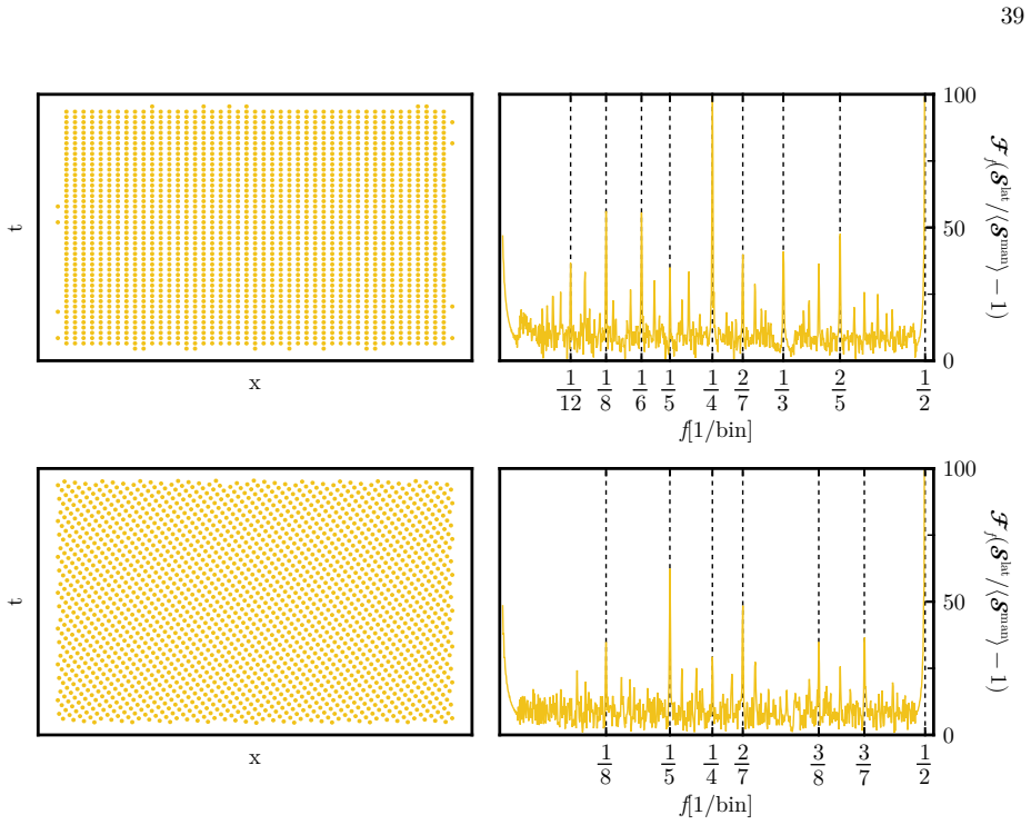
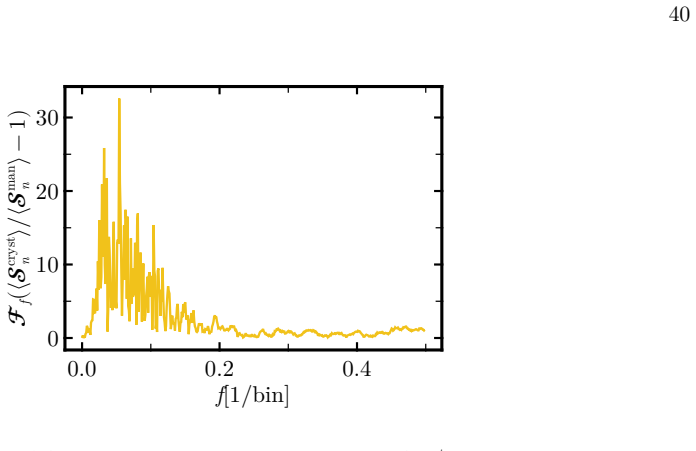
- Non-manifoldlike examples such as Lorentzian quasicrystals are distinguishable from lattices and layered orders.
- The method works for the tested volume range without requiring continuum-geometry calculations.
Where Pith is reading between the lines
- If the observables remain stable at volumes relevant to continuum recovery, they could be used to sample the measure over causal sets in numerical quantum-gravity simulations.
- The same statistics might serve as quick filters when generating random causal sets for other discrete-gravity models.
- Extending the test to ensembles drawn directly from the full configuration space (rather than hand-picked classes) would check whether the nine examples capture the main structural distinctions.
- Combinations of the three observables could define a low-dimensional chart of causal-set space whose axes have direct graph-theoretic meaning.
Load-bearing premise
The nine chosen classes are representative of the full configuration space and the distinguishing power of the observables survives at larger volumes and under coarse graining.
What would settle it
Finding substantial overlap between the observable values of two different classes or large fluctuations inside one class when the causal sets are scaled to higher volume would falsify the claim.
Figures
read the original abstract
The configuration space of causal sets is vast. It is a critical goal to map out this space. Here, we take a practical step towards this goal. We investigate nine classes of causal sets, most of them not studied before. These include manifoldlike causal sets with inhomogeneous Ricci curvature, both topologically trivial and nontrivial. We also study classes of non-manifoldlike causal sets, including lattices, layered orders as well as Lorentzian quasicrystals. Finally, we study classes of causal sets that are not manifoldlike, but are expected to become manifoldlike under a suitable coarse-graining process. We use this broad range of distinct classes of causal sets as a testbed for observables. Rather than focusing on continuum-geometry inspired observables, such as curvature invariants, which often exhibit large fluctuations and are computationally very expensive, we focus on graph observables, including some observables that constitute subgraph statistics and some that are global. We find that three observables, namely the link degree distribution, the eigenvalues of the graph Laplacian of the symmetrized Hasse diagram and the recently proposed abundance of causal intervals, can distinguish between the distinct classes of causal sets. This is made possible by the small fluctuations that these observables have in most classes.
Editorial analysis
A structured set of objections, weighed in public.
Referee Report
Summary. The paper claims that three graph observables—the link degree distribution, the eigenvalues of the graph Laplacian of the symmetrized Hasse diagram, and the abundance of causal intervals—can distinguish nine classes of causal sets (manifoldlike with inhomogeneous Ricci curvature, both topologically trivial and nontrivial; non-manifoldlike including lattices, layered orders, and Lorentzian quasicrystals; and classes expected to become manifoldlike under coarse-graining) because these observables exhibit small within-class fluctuations, in contrast to more expensive continuum-geometry observables.
Significance. If the distinguishing power is quantitatively verified and shown to be robust, the work offers a practical, computationally tractable route to charting causal-set configuration space using subgraph and global graph statistics. The breadth of the nine classes tested, including several not previously studied, is a positive feature that could help isolate which classes are viable for continuum recovery.
major comments (2)
- [Abstract] Abstract: the central claim that the three observables distinguish the classes via small fluctuations is stated without any quantitative data, error analysis, sampling protocol, or figures showing within-class variance versus inter-class separation, so the claim cannot be verified from the manuscript.
- [Main text (discussion of classes and observables)] The demonstration is performed only on finite-volume realizations of the nine classes; the manuscript does not test whether the reported small fluctuations and inter-class separation persist at substantially larger element counts or under the coarse-graining operations invoked for the final class of examples, which is load-bearing for the stated goal of mapping toward continuum recovery.
Simulated Author's Rebuttal
We are grateful to the referee for the positive assessment of the significance of our work and for the detailed comments that will help improve the manuscript. We respond to the major comments point by point below.
read point-by-point responses
-
Referee: [Abstract] Abstract: the central claim that the three observables distinguish the classes via small fluctuations is stated without any quantitative data, error analysis, sampling protocol, or figures showing within-class variance versus inter-class separation, so the claim cannot be verified from the manuscript.
Authors: We agree that the abstract would benefit from additional quantitative context to support the central claim. In the revised manuscript we will expand the abstract to include brief quantitative indicators of within-class fluctuations (e.g., standard deviations across realizations) and inter-class separations, together with references to the relevant figures and a short description of the sampling protocol. revision: yes
-
Referee: [Main text (discussion of classes and observables)] The demonstration is performed only on finite-volume realizations of the nine classes; the manuscript does not test whether the reported small fluctuations and inter-class separation persist at substantially larger element counts or under the coarse-graining operations invoked for the final class of examples, which is load-bearing for the stated goal of mapping toward continuum recovery.
Authors: The present study is restricted to finite-volume realizations in order to establish the distinguishing power of the three graph observables at computationally accessible scales. We acknowledge that verifying the persistence of the reported fluctuations and separations at substantially larger volumes and under explicit coarse-graining would strengthen the connection to continuum recovery. Such extensions are computationally demanding and lie outside the scope of the current work; we will add an explicit discussion of this limitation and of planned future investigations in the revised manuscript. revision: partial
Circularity Check
No circularity: empirical distinction via direct computation on chosen classes
full rationale
The paper selects nine classes of causal sets, generates realizations, and computes three graph observables (link degree distribution, Laplacian eigenvalues of symmetrized Hasse diagram, causal interval abundance). It reports that small within-class fluctuations permit inter-class distinction. This is a direct empirical observation on finite samples, not a derivation, fit, or self-referential definition. No equations reduce the reported distinctions to inputs by construction, no parameters are fitted and then relabeled as predictions, and no load-bearing self-citations or uniqueness theorems are invoked to force the result. The central claim remains independent of the inputs and is self-contained as an observational survey.
Axiom & Free-Parameter Ledger
Reference graph
Works this paper leans on
-
[1]
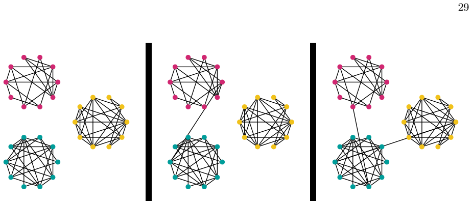
pants” topologies significantly reduce the number of links of a given element within one “pant leg
Physical interpretation For the link matrix,d in andd out count immediate predecessors and successors. The link matrix probes local connectivity at the discreteness scale and is sensitive to local geometric as well as topological features and also boundary effects. This is reflected in the link degree distribution. Link-degree distributions are sensitive ...
-
[2]
spectrum
Mathematical definition Given the causal intervalI[e i, ej] between any pair of elementse i ≺e j in a causal set, we can consider those intervals of cardinalitym, where we remind the reader that we defined the interval I[e i, ej] withe i ≺ ∗ej to have cardinality 2. We then define the interval abundance, also called “spectrum” in [27] for a causal setCwit...
-
[3]
nearest-neighbors
Physical interpretation The interval abundance is a simple example of subgraph statistics, because it counts the relative abundance of sub-causal sets of a given size, which are selected due to their causality properties. Causal intervals are building blocks of the d’Alembertian in a causal set [61, 80], because they can be understood as collecting the “n...
2048
-
[4]
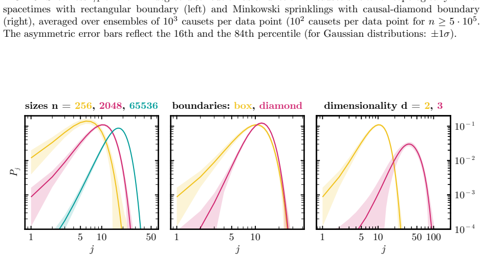
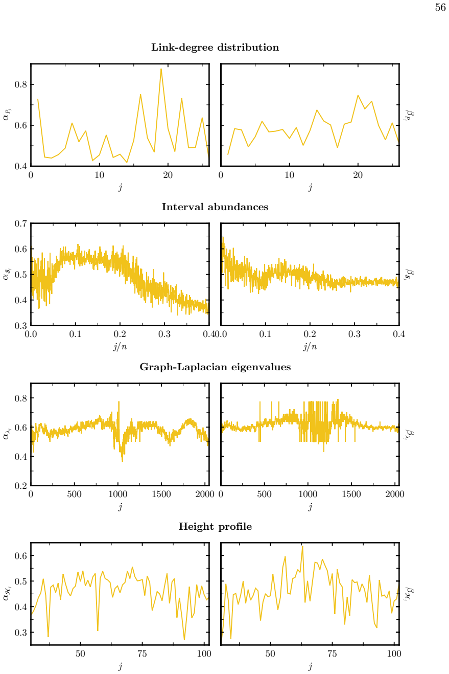
Link-degree distribution We show how the link-degree distribution varies in Fig. 17. All three changes shift the maximum of the link distribution to larger values. Further, the distribution becomes less skewed. A change in the boundary type from a box-boundary to a causal-diamond boundary changes the relative number of elements close to the boundary and t...
-
[5]
Interval abundances We examine how the interval abundances vary in Fig. 18. We find that with our normalization, the interval abundances are largely size- and boundary-independent. The dimensionality, however, has a very strong imprint leading to many more small intervals and fewer large intervals. This effect can be clearly differentiated from the featur...
-
[6]
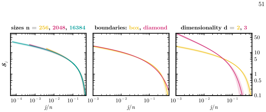
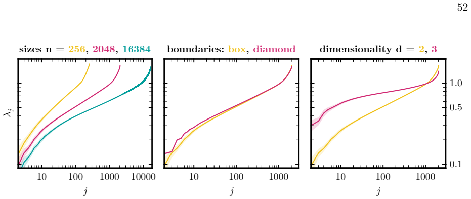
Graph-Laplacian eigenvalues We summarize how the graph-Laplacian eigenvalues vary in Fig. 19. The eigenvalues generally decrease with increasing causet size. This indicates that large causets have larger, more loosely connected subregions, and are less layered. While this reflects the natural inverse square scaling of the eigenvalues of geometric Laplacia...
2048
-
[7]
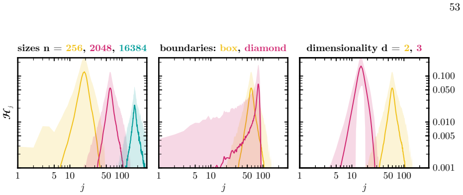
Height profile We show how the height profile varies in Fig. 20. The causal-diamond height profile clearly has a different shape compared to a rectangular boundary, showing how sensitive the height profile is to boundary modifications. Besides, the height profile is shifted towards larger heights for larger linear extent in one dimensionn 1/d, and becomes...
2048
-
[8]
Suppression of non-manifold-like sets in the causal set path integral,
S. P. Loomis and S. Carlip, “Suppression of non-manifold-like sets in the causal set path integral,” Class.Quant.Grav.35(9, 2017)
2017
-
[9]
Entropy and the link action in the causal set path-sum,
A. Mathur, A. A. Singh, and S. Surya, “Entropy and the link action in the causal set path-sum,” Class.Quant.Grav.38(12, 2020)
2020
-
[10]
Path integral suppression of badly behaved causal sets,
P. Carlip, S. Carlip, and S. Surya, “Path integral suppression of badly behaved causal sets,”Class. Quant. Grav.40no. 8, (2023) 095004, arXiv:2209.00327 [gr-qc]
-
[11]
The Einstein–Hilbert action for entropically dominant causal sets,
P. Carlip, S. Carlip, and S. Surya, “The Einstein–Hilbert action for entropically dominant causal sets,”Class. Quant. Grav.41no. 14, (2024) 145005, arXiv:2311.18238 [gr-qc]
-
[12]
Causal sets and an emerging continuum,
S. Carlip, “Causal sets and an emerging continuum,”Gen. Rel. Grav.56no. 8, (2024) 95, arXiv:2405.14059 [gr-qc]
-
[13]
Evidence for a Phase Transition in 2D Causal Set Quantum Gravity
S. Surya, “Evidence for a Phase Transition in 2D Causal Set Quantum Gravity,”Class. Quant. Grav.29(2012) 132001, arXiv:1110.6244 [gr-qc]
work page internal anchor Pith review Pith/arXiv arXiv 2012
-
[14]
Finite Size Scaling in 2d Causal Set Quantum Gravity
L. Glaser, D. O’Connor, and S. Surya, “Finite size scaling in 2d causal set quantum gravity,”Class. Quant. Grav.35no. 4, (2018) 045006, arXiv:1706.06432 [gr-qc]
work page internal anchor Pith review Pith/arXiv arXiv 2018
-
[15]
Dimensionally restricted causal set quantum gravity: examples in two and three dimensions,
W. J. Cunningham and S. Surya, “Dimensionally restricted causal set quantum gravity: examples in two and three dimensions,”Class. Quant. Grav.37no. 5, (2020) 054002, arXiv:1908.11647 [gr-qc]
-
[16]
Statistical geometry,
J. Myrheim, “Statistical geometry,” tech. rep., CERN, Geneva, 1978
1978
-
[17]
D. A. Meyer,The dimension of causal sets,The dimension of causal sets, 1988. PhD thesis, Massachusetts Institute of Technology
1988
-
[18]
The manifold dimension of a causal set: Tests in conformally flat space-times,
D. D. Reid, “The manifold dimension of a causal set: Tests in conformally flat space-times,” Phys.Rev.D67(1, 2003)
2003
-
[19]
Spectral dimension in causal set quantum gravity,
A. Eichhorn and S. Mizera, “Spectral dimension in causal set quantum gravity,”Class.Quant.Grav. 31(11, 2013)
2013
-
[20]
Spectral dimension on spatial hypersurfaces in causal set quantum gravity,
A. Eichhorn, S. Surya, and F. Versteegen, “Spectral dimension on spatial hypersurfaces in causal set quantum gravity,”Class.Quant.Grav.36(5, 2019)
2019
-
[21]
A Complete Set of Riemann Invariants,
E. Zakhary and C. B. G. Mcintosh, “A Complete Set of Riemann Invariants,”Gen. Rel. Grav.29 no. 5, (1997) 539–581
1997
-
[22]
The Scalar Curvature of a Causal Set
D. M. T. Benincasa and F. Dowker, “The Scalar Curvature of a Causal Set,”Phys. Rev. Lett.104 (2010) 181301, arXiv:1001.2725 [gr-qc]
work page internal anchor Pith review Pith/arXiv arXiv 2010
-
[23]
Higher-order curvature operators in causal set quantum gravity,
G. P. de Brito, A. Eichhorn, and C. Pfeiffer, “Higher-order curvature operators in causal set quantum gravity,”Eur. Phys. J. Plus138no. 7, (2023) 592, arXiv:2301.13525 [gr-qc]
-
[24]
Science 298, 5594 (2002), 824–827
R. Milo,et al., “Network motifs: Simple building blocks of complex networks,”Science298 no. 5594, (2002) 824–827, https://www.science.org/doi/pdf/10.1126/science.298.5594.824
-
[25]
N. M. Kriege, F. D. Johansson, and C. Morris, “A survey on graph kernels,”Applied Network Science5no. 1, (2020) 6, arXiv:1903.11835 [cs.LG]. 58
-
[26]
QuantumGrav,
K. T. Le, H. Mack, and F. Wagner, “QuantumGrav,”.https://github.com/ssciwr/QuantumGrav. GitHub repository, 2026
2026
-
[27]
CausalSetZoology,
F. Wagner, “CausalSetZoology,”.https://github.com/causal-wagner/CausalSetZoology. GitHub repository, 2026
2026
-
[28]
CausalSets.jl: A package for numerical simulations of the causal set approach to quantum gravity.,
V. A. Hollmeier, “CausalSets.jl: A package for numerical simulations of the causal set approach to quantum gravity.,”.https://codeberg.org/cyclopentane/CausalSets.jl. Codeberg repository, 2025
2025
-
[29]
Onset of the Asymptotic Regime for Finite Orders
J. Henson, D. P. Rideout, R. D. Sorkin, and S. Surya, “Onset of the Asymptotic Regime for Finite Orders,” arXiv:1504.05902 [math.CO]
work page internal anchor Pith review Pith/arXiv arXiv
-
[30]
Asymptotic enumeration of partial orders on a finite set,
D. J. Kleitman and B. L. Rothschild, “Asymptotic enumeration of partial orders on a finite set,” Transactions of the American Mathematical Society205(1975) 205–220
1975
-
[31]
Asymptotic enumeration of partially ordered sets,
D. Dhar, “Asymptotic enumeration of partially ordered sets,”Pacific Journal of Mathematics90 no. 2, (1980) 299–305
1980
-
[32]
Phase transitions in the evolution of partial orders,
H. J. Pr¨ omel, A. Steger, and A. Taraz, “Phase transitions in the evolution of partial orders,”Journal of Combinatorial Theory, Series A94(2001) 230–275
2001
-
[33]
Statistical Lorentzian geometry and the closeness of Lorentzian manifolds
L. Bombelli, “Statistical Lorentzian geometry and the closeness of Lorentzian manifolds,”J. Math. Phys.41(2000) 6944–6958, arXiv:gr-qc/0002053
work page internal anchor Pith review Pith/arXiv arXiv 2000
-
[34]
Closeness function on coarse grained Lorentzian geometries,
S. Surya, “Closeness function on coarse grained Lorentzian geometries,”Phys. Rev. D113no. 2, (2026) 024034, arXiv:2510.19403 [gr-qc]. [28]H.E.S.S.Collaboration, A. Abramowskiet al., “Search for Lorentz Invariance breaking with a likelihood fit of the PKS 2155-304 Flare Data Taken on MJD 53944,”Astropart. Phys.34(2011) 738–747, arXiv:1101.3650 [astro-ph.HE...
-
[35]
Space-Time as a Causal Set,
L. Bombelli, J. Lee, D. Meyer, and R. Sorkin, “Space-Time as a Causal Set,”Phys. Rev. Lett.59 (1987) 521–524
1987
-
[36]
Discreteness without symmetry breaking: a theorem
L. Bombelli, J. Henson, and R. D. Sorkin, “Discreteness without symmetry breaking: A Theorem,” Mod. Phys. Lett. A24(2009) 2579–2587, arXiv:gr-qc/0605006. 59
work page internal anchor Pith review Pith/arXiv arXiv 2009
-
[37]
J. P. Boyd,Chebyshev and Fourier Spectral Methods. Dover Books on Mathematics. Dover Publications, Mineola, NY, second ed., 2001
2001
-
[38]
Onset of the Asymptotic Regime for (Uniformly Random) Finite Orders,
J. Henson, D. Rideout, R. D. Sorkin, and S. Surya, “Onset of the Asymptotic Regime for (Uniformly Random) Finite Orders,”Exper. Math.26no. 3, (2016) 253–266
2016
-
[39]
L. Boyle and S. Mygdalas, “Spacetime Quasicrystals,” arXiv:2601.07769 [hep-th]
-
[40]
The role of aesthetics in pure and applied mathematical research,
R. Penrose, “The role of aesthetics in pure and applied mathematical research,”Bull.Inst.Math.Appl. 10(1974) 266–271
1974
-
[41]
Metallic phase with long-range orientational order and no translational symmetry,
D. Shechtman, I. Blech, D. Gratias, and J. W. Cahn, “Metallic phase with long-range orientational order and no translational symmetry,”Phys. Rev. Lett.53(Nov, 1984) 1951–1953
1984
-
[42]
Quasicrystals: A new class of ordered structures,
D. Levine and P. J. Steinhardt, “Quasicrystals: A new class of ordered structures,”Physical Review Letters53(1984) 2477–2480
1984
-
[43]
Gr¨ unbaum and G
B. Gr¨ unbaum and G. C. Shephard,Tilings and patterns. Courier Dover Publications, 1987
1987
-
[44]
A guide to mathematical quasicrystals
M. Baake,A Guide to Mathematical Quasicrystals, pp. 17–48. Springer Berlin Heidelberg, Berlin, Heidelberg, 2002. arXiv:math-ph/9901014 [math-ph]
work page internal anchor Pith review Pith/arXiv arXiv 2002
-
[45]
Quasiperiodic patterns,
M. Duneau and A. Katz, “Quasiperiodic patterns,”Phys. Rev. Lett.54(Jun, 1985) 2688–2691
1985
-
[46]
The diffraction pattern of projected structures,
V. Elser, “The diffraction pattern of projected structures,”Acta Crystallographica Section A42 no. 1, (1986) 36–43, https://onlinelibrary.wiley.com/doi/pdf/10.1107/S0108767386099932
-
[47]
Baake and U
M. Baake and U. Grimm,Aperiodic Order. Volume 1: A Mathematical Invitation. Cambridge University Press, 2013
2013
-
[48]
Diffraction of stochastic point sets: Explicitly computable examples
M. Baake, M. Birkner, and R. V. Moody, “Diffraction of stochastic point sets: Explicitly computable examples,”Communications in Mathematical Physics293no. 3, (2010) 611–660, arXiv:0803.1266 [math-ph]
work page internal anchor Pith review Pith/arXiv arXiv 2010
-
[49]
Hyperuniformity and non-hyperuniformity of quasicrystals,
M. Bj¨ orklund and T. Hartnick, “Hyperuniformity and non-hyperuniformity of quasicrystals,”arXiv e-prints(Oct., 2022) arXiv:2210.02151, arXiv:2210.02151 [math-ph]
-
[50]
Stable Homology as an Indicator of Manifoldlikeness in Causal Set Theory
S. Major, D. Rideout, and S. Surya, “Stable Homology as an Indicator of Manifoldlikeness in Causal Set Theory,”Class. Quant. Grav.26(2009) 175008, arXiv:0902.0434 [gr-qc]
work page internal anchor Pith review Pith/arXiv arXiv 2009
-
[51]
Exploring Quantum Spacetime with Topological Data Analysis,
J. van der Duin, R. Loll, M. Schiffer, and A. Silva, “Exploring Quantum Spacetime with Topological Data Analysis,” arXiv:2510.05693 [hep-th]
-
[52]
Quantum gravity and effective topology,
J. van der Duin, R. Loll, M. Schiffer, and A. Silva, “Quantum gravity and effective topology,”Eur. Phys. J. C86no. 2, (2026) 102, arXiv:2510.05695 [hep-th]
-
[53]
Towards coarse graining of discrete Lorentzian quantum gravity
A. Eichhorn, “Towards coarse graining of discrete Lorentzian quantum gravity,”Class. Quant. Grav. 35no. 4, (2018) 044001, arXiv:1709.10419 [gr-qc]
work page internal anchor Pith review Pith/arXiv arXiv 2018
-
[54]
Dimensional reduction in causal set gravity,
S. Carlip, “Dimensional reduction in causal set gravity,”
-
[55]
Dimensional reduction in manifold-like causal sets,
J. Abajian and S. Carlip, “Dimensional reduction in manifold-like causal sets,”Phys.Rev.D97(10,
-
[56]
Echoes of asymptotic silence in causal set quantum gravity,
A. Eichhorn, S. Mizera, and S. Surya, “Echoes of asymptotic silence in causal set quantum gravity,” Class.Quant.Grav.34(3, 2017) . 60
2017
-
[57]
Estimating the manifold dimension of causal sets,
F. Ashmead and D. D. Reid, “Estimating the manifold dimension of causal sets,”Handbook of Quantum Gravity(2024) 1–21
2024
-
[58]
The random discrete action for 2-dimensional spacetime,
D. M. T. Benincasa, F. Dowker, and B. Schmitzer, “The random discrete action for 2-dimensional spacetime,”Class.Quant.Grav.28(11, 2010)
2010
-
[59]
Discrete geometry of a small causal diamond,
M. Roy, D. Sinha, and S. Surya, “Discrete geometry of a small causal diamond,”Phys.Rev.D87(2,
-
[60]
Particle propagators on discrete spacetime,
S. Johnston, “Particle propagators on discrete spacetime,”Class.Quant.Grav.25(10, 2008)
2008
-
[61]
Scalar field theory on a causal set in histories form,
R. D. Sorkin, “Scalar field theory on a causal set in histories form,”J.Phys.Conf.Ser.306(2011)
2011
-
[62]
Causal set d’alembertians for various dimensions,
F. Dowker and L. Glaser, “Causal set d’alembertians for various dimensions,”Class.Quant.Grav.30 (10, 2013)
2013
-
[63]
A closed form expression for the causal set d’alembertian,
L. Glaser, “A closed form expression for the causal set d’alembertian,”Class.Quant.Grav.31(5,
-
[64]
Generalized causal set d‘alembertians,
S. Aslanbeigi, M. Saravani, and R. D. Sorkin, “Generalized causal set d‘alembertians,”JHEP06 (2014) 024
2014
-
[65]
Correction terms for propagators and d’alembertians due to spacetime discreteness,
S. Johnston, “Correction terms for propagators and d’alembertians due to spacetime discreteness,” Class.Quant.Grav.32(9, 2015)
2015
-
[66]
The continuum limit of a 4-dimensional causal set scalar d’alembertian,
A. Belenchia, D. M. Benincasa, and F. Dowker, “The continuum limit of a 4-dimensional causal set scalar d’alembertian,”Class.Quant.Grav.33(12, 2016)
2016
-
[67]
Towards spectral geometry for causal sets,
Y. K. Yazdi and A. Kempf, “Towards spectral geometry for causal sets,”Class.Quant.Grav.34(3,
-
[68]
Scalar field green functions on causal sets,
S. N. Ahmed, F. Dowker, and S. Surya, “Scalar field green functions on causal sets,” Class.Quant.Grav.34(5, 2017)
2017
-
[69]
Combinatorial interpretation of the coefficients of the causal set d’alembertian,
K. Yeats, “Combinatorial interpretation of the coefficients of the causal set d’alembertian,”Classical and Quantum Gravity42(3, 2025) 145003
2025
-
[70]
Local d’alembertian for causal sets,
M. Bogu˜ n´ a and D. Krioukov, “Local d’alembertian for causal sets,”
-
[71]
Retarded causal set propagator in 2d anti de-sitter spacetime,
A. Kastrati and H. Hinrichsen, “Retarded causal set propagator in 2d anti de-sitter spacetime,”
-
[72]
On recovering continuum topology from a causal set,
S. Major, D. Rideout, and S. Surya, “On recovering continuum topology from a causal set,” J.Math.Phys.48(2007)
2007
-
[73]
Causal set topology,
S. Surya, “Causal set topology,”Theor.Comput.Sci.405(10, 2008) 188–197
2008
-
[74]
Path length distribution in two-dimensional causal sets,
M. Aghili, L. Bombelli, and B. B. Pilgrim, “Path length distribution in two-dimensional causal sets,” Eur.Phys.J.C78(9, 2018) 744
2018
-
[75]
Manifold properties from causal sets using chains,
J. Kambor and X. Nomaan, “Manifold properties from causal sets using chains,”Class.Quant.Grav. 38(1, 2020)
2020
-
[76]
On the continuum limit of benincasa-dowker-glaser causal set action,
L. Machet and J. Wang, “On the continuum limit of benincasa-dowker-glaser causal set action,” Class.Quant.Grav.38(7, 2020)
2020
-
[77]
Boundary contributions in the causal set action,
F. Dowker, “Boundary contributions in the causal set action,”Gen.Rel.Grav.38(4, 2021)
2021
-
[78]
Local structure of sprinkled causal sets,
C. J. Fewster, E. Hawkins, C. Minz, and K. Rejzner, “Local structure of sprinkled causal sets,” 61 Phys.Rev.D103(4, 2021)
2021
-
[79]
Benincasa-dowker causal set actions by quantum counting,
S. A. Adamson and P. Wallden, “Benincasa-dowker causal set actions by quantum counting,”
-
[80]
The causal set approach to quantum gravity,
S. Surya, “The causal set approach to quantum gravity,”Living Rev. Rel.22no. 1, (2019) 5, arXiv:1903.11544 [gr-qc]
discussion (0)
Sign in with ORCID, Apple, or X to comment. Anyone can read and Pith papers without signing in.