pith. sign in

arxiv: 2605.30412 · v2 · pith:TE5ZJUREnew · submitted 2026-05-28 · 🌌 astro-ph.IM · astro-ph.CO· astro-ph.GA

Choosing the right MCMC sampler: a systematic benchmark of gradient-free methods

Pith reviewed 2026-06-29 00:21 UTC · model grok-4.3

classification 🌌 astro-ph.IM astro-ph.COastro-ph.GA
keywords MCMCdifferential evolutionsampler comparisonastrophysical inferenceRosenbrock functionNeal's funnelmultimodal likelihoodacceptance rate tuning
0
0 comments X

The pith

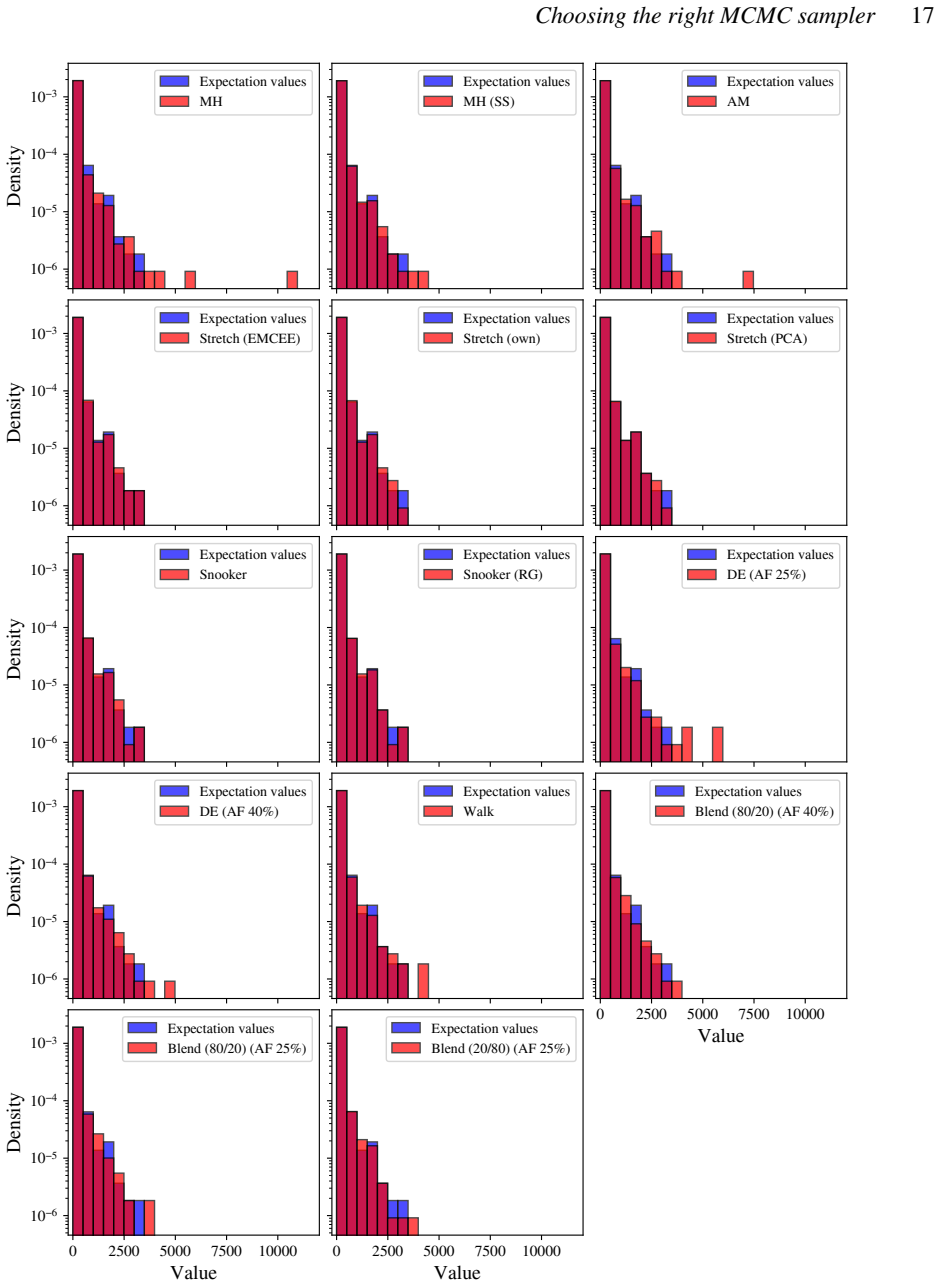
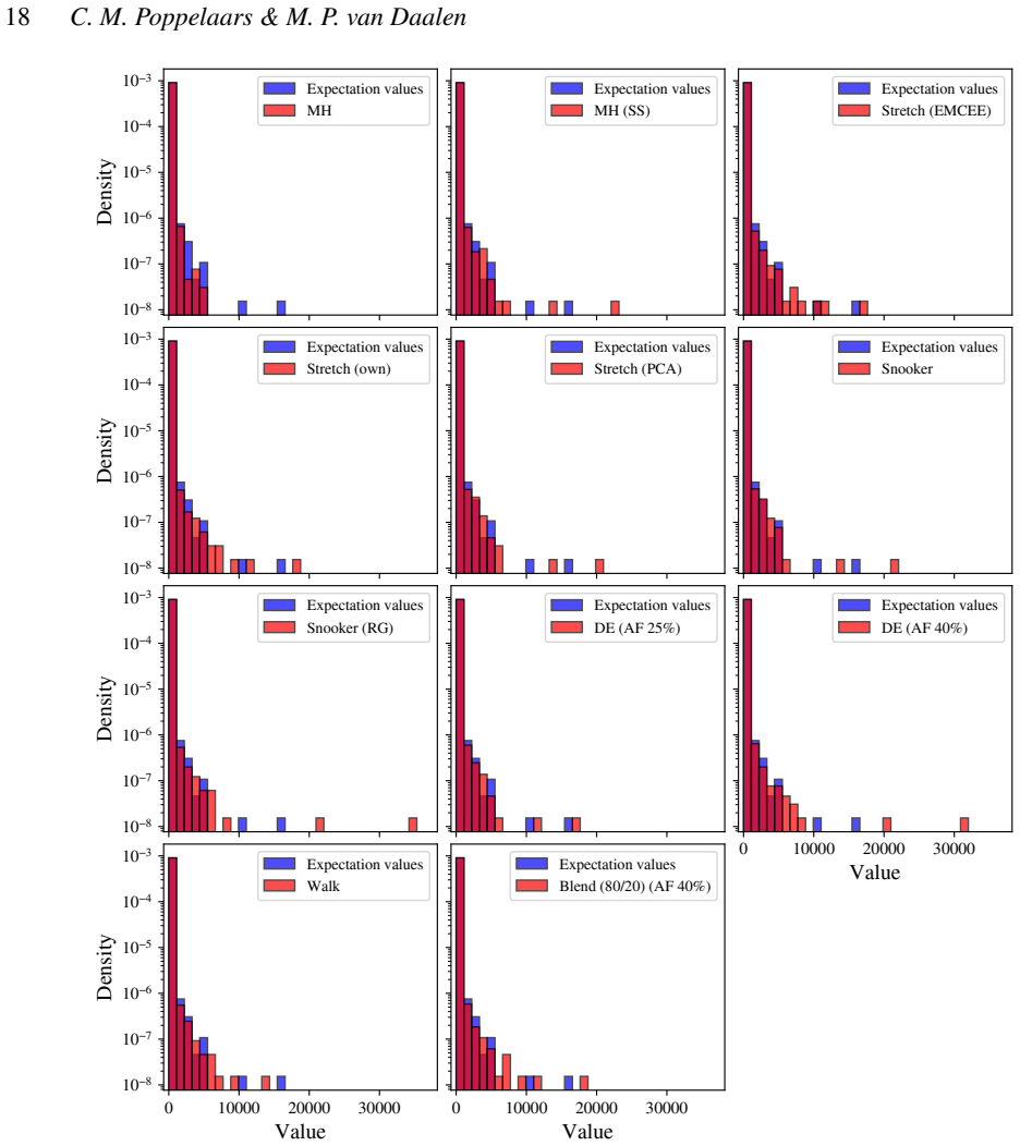
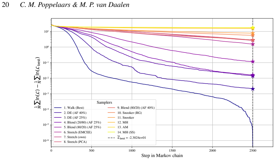
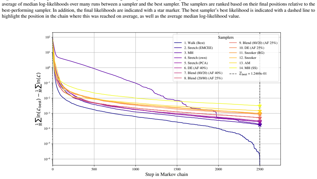
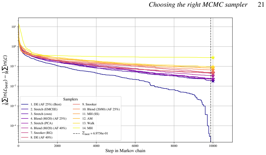
Differential evolution MCMC, tuned to 25 percent acceptance, outperforms stretch, walk, snooker and hybrid moves on the chosen test functions.

A machine-rendered reading of the paper's core claim, the machinery that carries it, and where it could break.

The paper benchmarks several gradient-free MCMC samplers on the Rosenbrock function, Neal's funnel, and Gaussian random landscapes in three to eight dimensions. It measures performance by ergodicity, robustness to starting points, and final likelihood values reached. The results indicate that a differential evolution proposal tuned to a 25 percent acceptance rate produces better mixing and higher likelihoods than the other tested moves, including two new variants introduced in the work. The authors also show that a post-sampling optimization step improves the best-found likelihood, with larger gains in higher dimensions. These comparisons are offered as guidance for choosing samplers in astrophysical inference problems.

Core claim

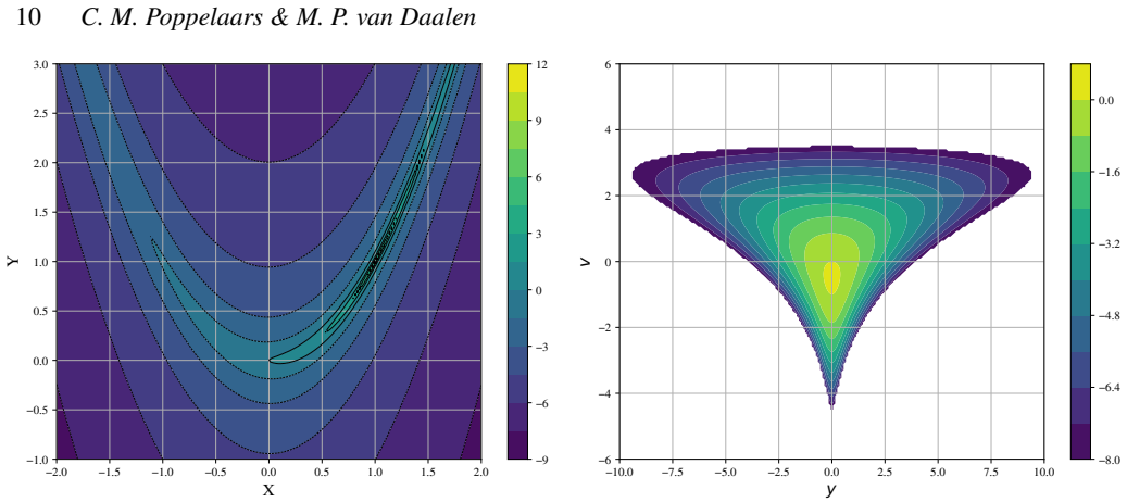
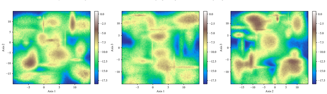
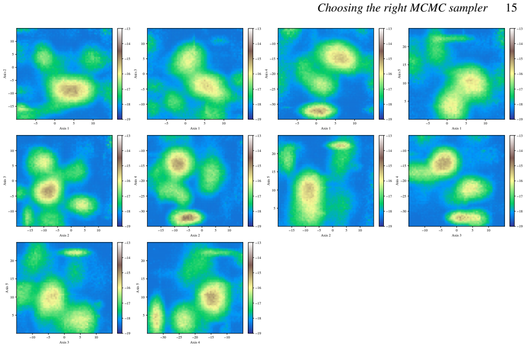
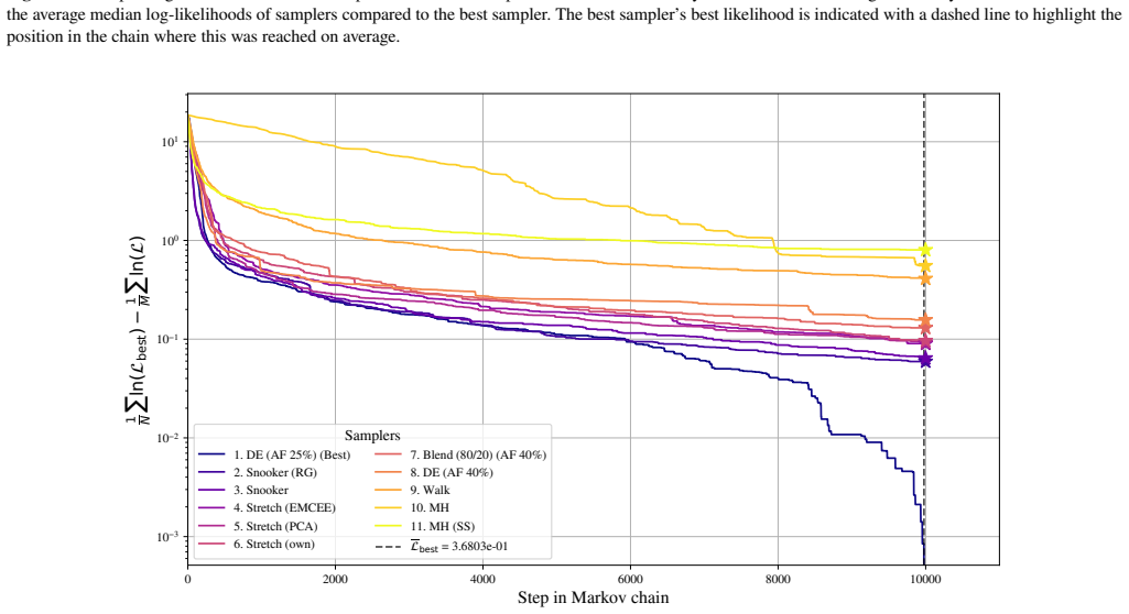
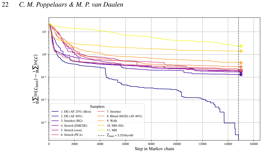
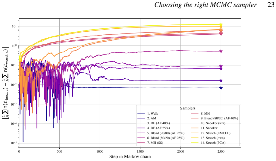
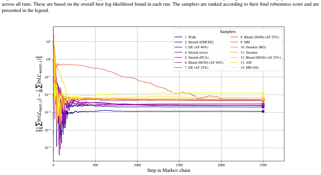
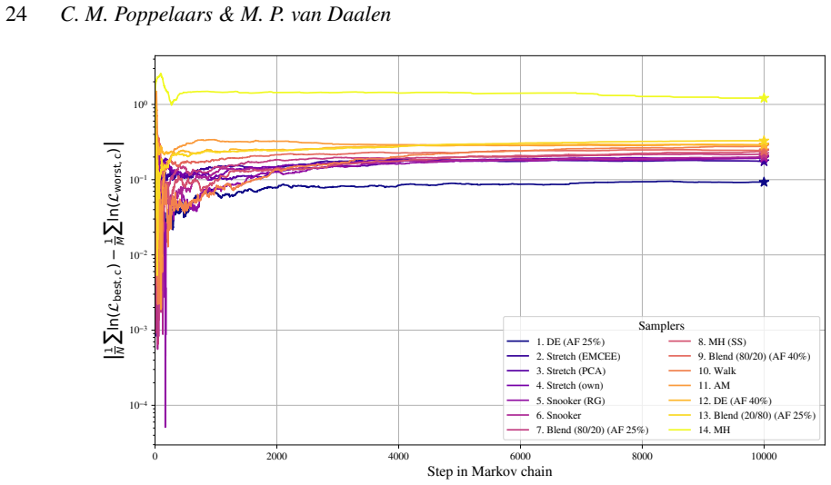
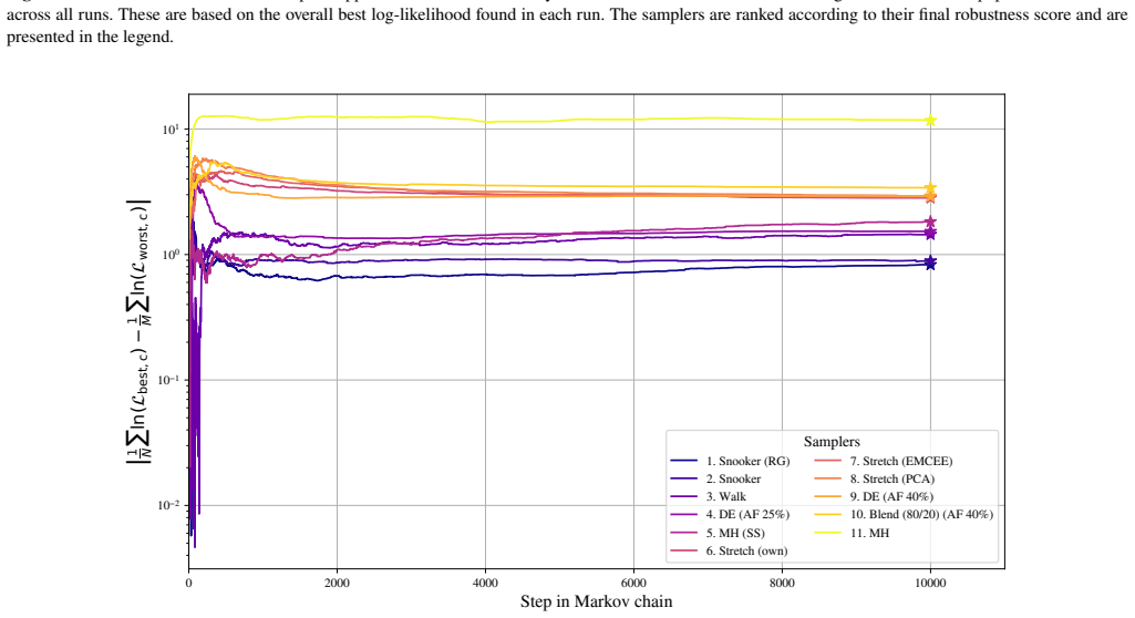
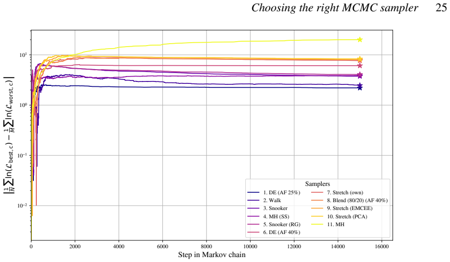
When the differential evolution move is tuned to a target acceptance fraction of 25 percent, it produces higher ergodicity, greater robustness across starting positions, and better likelihood performance than the stretch move, walk move, snooker move, PCA-modified stretch move, and hybrid blend move on the Rosenbrock, Neal's funnel, and multimodal Gaussian random landscapes.

What carries the argument

The differential evolution proposal step, adjusted to maintain a 25 percent acceptance rate, used inside an otherwise standard Metropolis-Hastings framework.

If this is right

  • Astrophysical codes that currently default to stretch or walk moves could switch to differential evolution with a 25 percent acceptance target to reach higher-likelihood regions in fewer steps.
  • The post-sampling optimization refinement becomes more valuable as dimension increases, suggesting it should be applied routinely after any MCMC run in problems with five or more parameters.
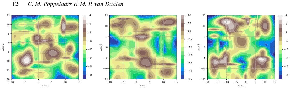
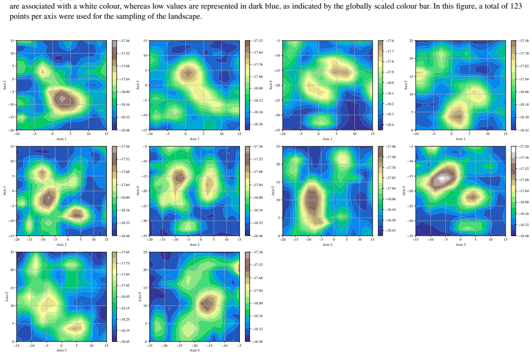
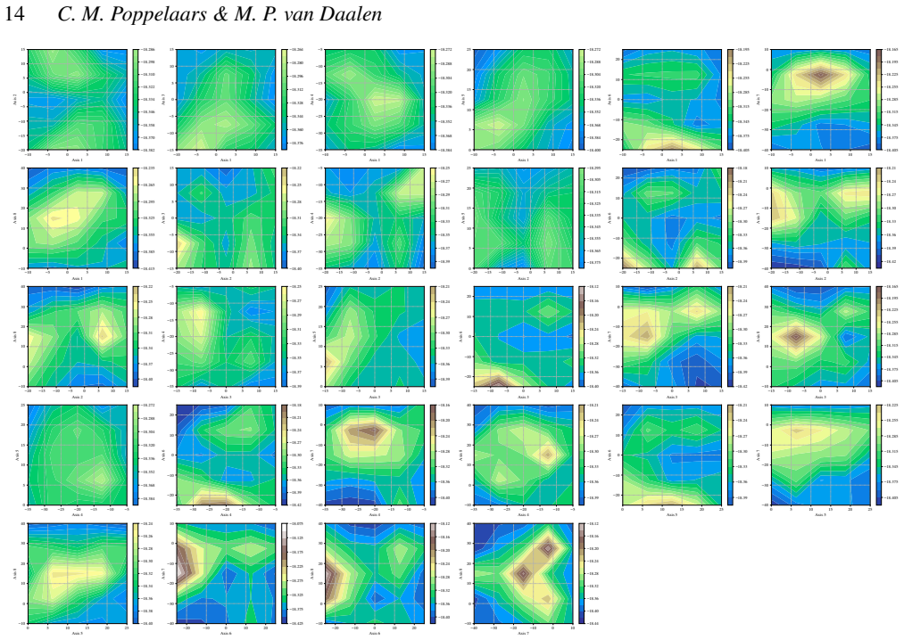
  • Reconstruction of likelihood surfaces via quadtree from the sampled points offers a practical way to visualize and diagnose sampling quality without additional model evaluations.
  • The relative ordering of samplers may shift if the target acceptance rate is left at its default value instead of being tuned to 25 percent.

Where Pith is reading between the lines

These are editorial extensions of the paper, not claims the author makes directly.

  • If the performance ordering holds on real data, many existing MCMC pipelines in astronomy could reduce their burn-in time by adopting the tuned differential evolution move without changing any other part of the code.
  • The same benchmark protocol could be applied to gradient-based samplers such as Hamiltonian Monte Carlo to test whether the advantage persists when gradients are available.

Load-bearing premise

The Rosenbrock, Neal's funnel, and low-dimensional Gaussian random fields capture the essential difficulties of the multimodal, high-dimensional likelihood surfaces that arise in actual astrophysical data analysis.

What would settle it

Run the same suite of samplers on a real eight-or-higher-dimensional astrophysical posterior, such as a weak-lensing or exoplanet transit fit, and record whether the tuned differential evolution chain still reaches the highest likelihood and mixes fastest.

Figures

Figures reproduced from arXiv: 2605.30412 by Colin M. Poppelaars, Marcel P. van Daalen.

Figure 1
Figure 1. Figure 1: An illustration of a Markov chain. The chain starts from an initial position, from which proposals are created. Once a proposal is accepted based on the acceptance criterion, the sample is added to the chain. This process is repeated for 𝑁 times until the chain length is reached or if another termination cause has been reached. Here 𝑁 = 5. this initial phase, the chain is expected to have converged suffici… view at source ↗
Figure 2
Figure 2. Figure 2: A Gaussian Metropolis-Hastings move for current chain 𝑋® 𝑖 . The move is based on centring a Gaussian around the current position 𝑋® 𝑖 with a standard deviation of 𝜎. From this, a new point is sampled, 𝑋® 𝑖 new . et al. (1996); Roberts et al. (1997); Haario et al. (1999); Roberts & Rosenthal (2001); Haario et al. (2001); Atchadé & Rosenthal (2005); Brooks et al. (2011a). Despite the simplicity of the MH al… view at source ↗
Figure 3
Figure 3. Figure 3: An adaptive Metropolis move for chain 𝑋® 𝑖 . Initially, before 𝑡 = 𝑡0, we sample the 𝑋® 𝑖 new from the initial Gaussian distribution with covariance 𝐶0. Starting from 𝑡0, we use the empirical covariance 𝐶𝑡 . This adaptive covariance can increase or decrease the width of the Gaussian distribution. For this figure, we present an increased width. other walkers, the algorithm inherently adapts to the local geo… view at source ↗
Figure 4
Figure 4. Figure 4: A stretch move for current chain 𝑋® 𝑖 . The black dot represents the reference walker 𝑋® 𝑗 that is taken from the complementary ensemble of walkers. The stretch move stretches the difference between walkers 𝑋® 𝑖 and 𝑋® 𝑗 by a factor of 𝑍, as seen in equation (9), where 𝑍 is obtained by equation (10). From this move, we arrive at the new position, 𝑋® 𝑖 new [PITH_FULL_IMAGE:figures/full_fig_p006_4.png] view at source ↗
Figure 5
Figure 5. Figure 5: A walk move for current chain 𝑋® 𝑖 . The black and grey dots represent the complementary ensemble. The black dots mark the chains used from the complement for this walk move, i.e. |𝑆| = 4. The sample mean of these points is given by 𝑋¯ 𝑠. From this, we construct the covariance matrix 𝐶, which is used to propose the new point 𝑋® 𝑖 new by centring a normal distribution about 𝑋® 𝑖 with covariance 𝐶. This resu… view at source ↗
Figure 6
Figure 6. Figure 6: A Differential Evolution (DE) move for current walker 𝑋® 𝑖 . The blue and grey dots represent the walkers from the complementary ensemble. The blue dots are the reference walkers that are sampled at random from the ensemble, from which we determine the displacement that is scaled and added to 𝑋® 𝑖 to arrive at the proposal 𝑋® 𝑖 new . acceptance criterion, equation (1), ensuring that it satisfies detailed b… view at source ↗
Figure 8
Figure 8. Figure 8: A blend move for current chain 𝑋® 𝑖 . The blend move combines the proposal moves of the stretch, equation (9), and the differential evolution (DE) move, equation (15). The grey, blue, and black dots correspond to the complementary ensemble from which we sample the random walkers 𝑗, 𝑘, and 𝑙. From walker 𝑗, we obtain the stretch proposal; from 𝑘 and 𝑙 we obtain the DE proposal. These proposals are then blen… view at source ↗
Figure 9
Figure 9. Figure 9: A Principal Component Analysis (PCA) stretch move for current chain 𝑋® 𝑖 . The PCA stretch move transforms the complementary ensemble to the PCA space and picks a random walker 𝑗 to propose the new position 𝑋®new 𝑖, PCA, using the transformed 𝑋® 𝑖 . This new position is then transformed back into the parameter space by the inverse PCA transform, such that we obtain 𝑋®new 𝑖 . determinant of the change of va… view at source ↗
Figure 10
Figure 10. Figure 10: The Rosenbrock likelihood landscape. The landscape exhibits a banana-like shaped region of interest where the log-likelihood is highest. Outside this region, the log-likelihood is lower. The global optimum is located at (1,1). with zero mean and a variance that grows or shrinks exponentially with 𝑣. The sampling process is given by: 𝑣 ∼ N (0 | 3), 𝑦 ∼ N  0 | exp  𝑣 2   . (28) As a result, the standard… view at source ↗
Figure 12
Figure 12. Figure 12: The projections of the log-likelihood landscape of the 3D test case. The contours highlight elevation changes in the log-likelihood values. High values are associated with a white colour, whereas low values are represented in dark blue, as indicated by the globally scaled colour bar. In this figure, a total of 123 points per axis were used for the sampling of the landscape. −10 −5 0 5 10 15 Axis 1 −20 −15… view at source ↗
Figure 13
Figure 13. Figure 13: As figure 12, but for the 5D test case, using 8 points per axis and showing pairwise combinations of dimensions [PITH_FULL_IMAGE:figures/full_fig_p012_13.png] view at source ↗
Figure 14
Figure 14. Figure 14: As figure 12, but for the 8D test case, using 5 points per axis and showing all pairwise axis combinations. −5 0 5 10 Axis 1 −15 −10 −5 0 5 10 Axis 2 −5 0 5 10 Axis 1 −10 −5 0 5 10 Axis 3 −15 −10 −5 0 5 10 Axis 2 −10 −5 0 5 10 Axis 3 −17.5 −15.0 −12.5 −10.0 −7.5 −5.0 −2.5 0.0 −17.5 −15.0 −12.5 −10.0 −7.5 −5.0 −2.5 0.0 −17.5 −15.0 −12.5 −10.0 −7.5 −5.0 −2.5 0.0 [PITH_FULL_IMAGE:figures/full_fig_p014_14.png] view at source ↗
Figure 15
Figure 15. Figure 15: Reconstructed log-likelihood landscape of the 3D multiple Gaussian test case as shown in figure 12, using a quadtree. The colour scaling reflects the minimum and maximum log-likelihood values from the samples. The maximal depth of the quadtree used here is set at 7. 4 SAMPLER PERFORMANCE 4.1 Measuring the performance of a sampler Having introduced the various samplers in section 2 and the toy models in se… view at source ↗
Figure 16
Figure 16. Figure 16: As figure 15, but for the 5D test case with projections shown in figure 13. A maximal quadtree depth of 6 is used. The colour scale has been manually adjusted to span values from −19 to −13 for improved visibility. Isolated islands reflect the multimodal nature of the landscape. of multiple runs and visualising the progression of their best median log-likelihood values, we gain insight into how quickly an… view at source ↗
Figure 17
Figure 17. Figure 17: Ergodicity comparison between the expectation values of cells and the number of samples per cell for our 3D toy model. The data have been binned according to the Rice rule. The expectation values are plotted in blue, and the number of samples of each sampler is plotted in red. Each sampler has its unique subfigure, as highlighted by the label of the red colour bins. By overlaying the two, we identify the … view at source ↗
Figure 18
Figure 18. Figure 18: As figure 17, but for our 5D Gaussian toy model. The effective number of non-zero cells was 3 896, and the total number of cells was 59 049. 1 compared to the best sampler. We do not see this for Neal’s funnel; all samplers are within a log-likelihood ratio value of 10−2 . Notably, the snooker moves are ranked in both test cases near the lower end of the performance chart. The stretch moves cluster near e… view at source ↗
Figure 19
Figure 19. Figure 19: As figure 17, but for our 8D Gaussian toy model. The effective number of non-zero cells was 21 437, and the total number of cells was 1 679 616. fraction of 25% outperforms all samplers in each test case. Notably, the magnitude by which it outperforms the other moves increases with dimensionality. For 3D, the closest sampler is within a log￾likelihood difference of ∼ 2 · 10−2 , whereas for 5D this is ∼ 6 … view at source ↗
Figure 20
Figure 20. Figure 20: Sampler log-likelihood evolution over chain length compared to the best sampler of the Rosenbrock test case. Each curve is the difference of the average of median log-likelihoods over many runs between a sampler and the best sampler. The samplers are ranked based on their final positions relative to the best-performing sampler. In addition, the final likelihoods are indicated with a star marker. The best … view at source ↗
Figure 21
Figure 21. Figure 21: As figure 20, but for Neal’s funnel test case. 4.4 The robustness of samplers In addition to evaluating the average convergence behaviour of sam￾plers, we also assess theirrobustness. This metric captures the consis￾tency and reliability of a sampler across multiple independent runs, providing insight into its stability. Contrary to the previous metric, we store the chains with the highest and lowest achi… view at source ↗
Figure 22
Figure 22. Figure 22: Sampler log-likelihood evolution compared to the best sampler of the 3D Gaussian toy model. The curves are generated by the difference between the average median log-likelihoods of samplers compared to the best sampler. The best sampler’s best likelihood is indicated with a dashed line to highlight the position in the chain where this was reached on average. 0 2000 4000 6000 8000 10000 Step in Markov chai… view at source ↗
Figure 23
Figure 23. Figure 23: As figure 22, but for the 5D Gaussian toy model. particularly relevant when computational resources are limited and only a small number of chains can be run. In such settings, a robust sampler increases the possibility of achieving satisfactory conver￾gence in a single run. When interpreted in conjunction with the log-likelihood ratio evolution curves, this robustness metric helps to identify samplers tha… view at source ↗
Figure 24
Figure 24. Figure 24: As figure 22, but for the 8D Gaussian toy model. walk, adaptive Metropolis, and DE moves. Importantly, having a level curve is only a measure of good robustness whenever it is located at a low value. The worst-performing moves have a discrepancy above a log-likelihood of 1 in the Rosenbrock test case. In Neal’s funnel, this is at most 10−2 . Given both figures, we see that there exists an initial phase in… view at source ↗
Figure 25
Figure 25. Figure 25: Robustness curves for the samplers applied to the Rosenbrock test case. Each curve is constructed by using the worst and best populations of chains across all runs. These are based on the overall best log-likelihood found in each run. The samplers are ranked according to their final robustness score and are presented in the legend. 0 500 1000 1500 2000 2500 Step in Markov chain 10 −5 10 −4 10 −3 10 −2 10 … view at source ↗
Figure 26
Figure 26. Figure 26: As figure 25, but for Neal’s funnel test case. 4.5 Improving on the best set of parameters Once MCMC sampling has been performed for a given likelihood landscape, a natural follow-up question arises: “Can we further im￾prove upon the best parameter set identified during sampling?”. This question is particularly relevant for complex models, where even marginal improvements in the parameter set can yield no… view at source ↗
Figure 27
Figure 27. Figure 27: Robustness curves for the samplers applied to the 3D Gaussian toy model. The curves are constructed using the worst and best populations of chains across all runs. These are based on the overall best log-likelihood found in each run. The samplers are ranked according to their final robustness score and are presented in the legend. 0 2000 4000 6000 8000 10000 Step in Markov chain 10 −2 10 −1 10 0 10 1 | 1 … view at source ↗
Figure 28
Figure 28. Figure 28: As figure 27, but for the 5D toy model. Mead 1965). This is a derivative-free optimiser that is well-suited for noisy, non-smooth, or non-differentiable objective functions. It aims to climb the final stretch of the likelihood surface from a promising initial point, potentially uncovering a better-fitting parameter con￾figuration. In our experiments, we apply the DHS algorithm to our multimodal toy landsc… view at source ↗
Figure 29
Figure 29. Figure 29: As figure 27, but for the 8D toy model [PITH_FULL_IMAGE:figures/full_fig_p025_29.png] view at source ↗
read the original abstract

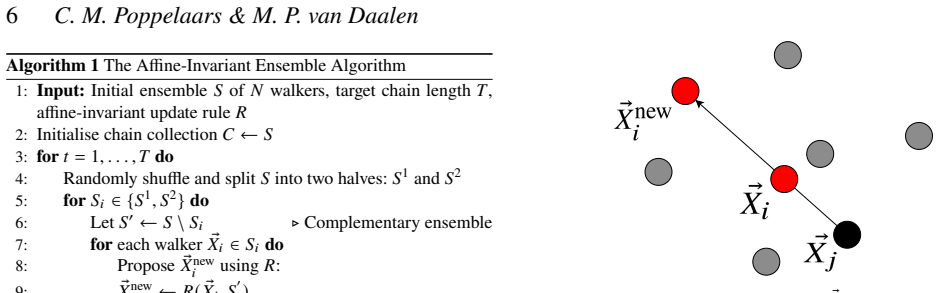
We present a set of metrics and methods for testing and comparing a range of modern gradient-free Markov Chain Monte Carlo (MCMC) samplers against the commonly used Metropolis-Hastings (MH) algorithm. The goal is to quantify key performance metrics, including sampler ergodicity, robustness and overall likelihood performance. To provide a controlled and interpretable testbed, we use the Rosenbrock function and Neal's funnel as representative unimodal cases, while Gaussian random likelihood landscapes in three, five, and eight dimensions serve as multimodal test scenarios. The samplers considered include affine-invariant moves from the literature, such as the stretch and walk moves, the differential evolution move, and the snooker move. We additionally introduce two novel variations: a modified stretch move that incorporates a Principal Component Analysis (PCA) transformation, and a hybrid blend move that combines features of both differential evolution and stretch dynamics. Beyond sampler evaluation, we demonstrate reconstructing likelihood landscapes from sampled points using a quadtree algorithm. Additionally, we explore the use of optimisation algorithms to refine the best parameter set in terms of its likelihood, and find consistent improvements in log-likelihood values, with the post-sampling gain becoming more significant in higher-dimensional problems. Our comparative results of sampler testing show that the differential evolution algorithm, when tuned to a target acceptance fraction of 25%, consistently outperforms all other samplers in terms of ergodicity, robustness, and likelihood performance.

Editorial analysis

A structured set of objections, weighed in public.

Desk editor's note, referee report, simulated authors' rebuttal, and a circularity audit. Tearing a paper down is the easy half of reading it; the pith above is the substance, this is the friction.

Referee Report

2 major / 1 minor

Summary. The manuscript benchmarks gradient-free MCMC samplers (affine-invariant stretch/walk/snooker moves, differential evolution, and two novel variants: PCA-modified stretch and hybrid blend) against Metropolis-Hastings. Using Rosenbrock and Neal's funnel as unimodal tests plus Gaussian random landscapes in 3/5/8 dimensions as multimodal cases, it reports that differential evolution tuned to 25% target acceptance consistently outperforms others in ergodicity, robustness, and likelihood. Additional contributions include quadtree reconstruction of likelihood landscapes from samples and post-sampling optimization that improves log-likelihood, with larger gains in higher dimensions.

Significance. If the reported ranking is robust, the work supplies a controlled comparison that could inform sampler choice in astrophysical inference pipelines. The novel moves and quadtree method are concrete methodological additions. However, the low-dimensional synthetic test suite limits the strength of any general recommendation for real problems.

major comments (2)
  1. [Abstract and test-function sections] Abstract and test-function sections: the central claim that differential evolution (25% acceptance) 'consistently outperforms all other samplers' rests entirely on Rosenbrock, Neal's funnel, and Gaussian random landscapes in ≤8 dimensions. These lack the parameter degeneracies, non-Gaussian tails, expensive forward models, and dimensionality (>10–20) typical of astrophysical posteriors; without additional tests on realistic cases or an explicit discussion of when the ranking may reverse, the comparative result does not support the broader claim for astro inference.
  2. [Sampler comparison and tuning description] Sampler comparison and tuning description: the 25% acceptance target is applied specifically to differential evolution, yet the manuscript does not report whether the other samplers (stretch, walk, snooker, novel variants) were subjected to equivalent acceptance-fraction tuning or left at default settings; this asymmetry could affect the reported ranking and must be clarified with explicit protocol details.
minor comments (1)
  1. The quadtree reconstruction and optimization sections would benefit from explicit pseudocode or a small worked example to make the methods reproducible.

Simulated Author's Rebuttal

2 responses · 0 unresolved

We thank the referee for their constructive and detailed comments. We address each major comment below, proposing targeted revisions to improve transparency and appropriately qualify our claims.

read point-by-point responses
  1. Referee: [Abstract and test-function sections] Abstract and test-function sections: the central claim that differential evolution (25% acceptance) 'consistently outperforms all other samplers' rests entirely on Rosenbrock, Neal's funnel, and Gaussian random landscapes in ≤8 dimensions. These lack the parameter degeneracies, non-Gaussian tails, expensive forward models, and dimensionality (>10–20) typical of astrophysical posteriors; without additional tests on realistic cases or an explicit discussion of when the ranking may reverse, the comparative result does not support the broader claim for astro inference.

    Authors: The test functions were selected to provide a controlled benchmark with analytically known properties, enabling isolation of sampler behavior on features such as multimodality and correlations. We acknowledge that these cases are lower-dimensional and lack the full complexity of typical astrophysical posteriors. In the revised manuscript we will expand the discussion (primarily in the conclusions) to explicitly address the limitations of the test suite, qualify the scope of the performance ranking, and note conditions under which the ranking could reverse in higher-dimensional or more realistic settings. revision: yes

  2. Referee: [Sampler comparison and tuning description] Sampler comparison and tuning description: the 25% acceptance target is applied specifically to differential evolution, yet the manuscript does not report whether the other samplers (stretch, walk, snooker, novel variants) were subjected to equivalent acceptance-fraction tuning or left at default settings; this asymmetry could affect the reported ranking and must be clarified with explicit protocol details.

    Authors: We agree that the tuning protocol must be stated explicitly. Differential evolution was tuned to a 25% target acceptance fraction following literature recommendations for that sampler, while the remaining samplers used their standard/default parameter settings. We will add a dedicated methods subsection (with an accompanying table) that reports the acceptance fractions achieved by each sampler and the precise tuning protocol applied, thereby removing any ambiguity about the comparison. revision: yes

Circularity Check

0 steps flagged

Empirical benchmark with no circular derivations

full rationale

The paper is a direct empirical comparison of MCMC sampler performance on fixed synthetic test functions (Rosenbrock, Neal's funnel, Gaussian random landscapes). Performance metrics are computed from the sampling runs themselves; the 25% acceptance target is a conventional tuning value, not a fitted parameter renamed as a prediction. No equations, self-citations, or ansatzes are invoked to derive the central ranking, so the reported outperformance stands as an independent experimental result on the chosen testbed.

Axiom & Free-Parameter Ledger

1 free parameters · 1 axioms · 0 invented entities

The benchmark relies on standard assumptions about MCMC convergence diagnostics and the representativeness of synthetic test functions; no new physical axioms or invented entities are introduced.

free parameters (1)
  • target acceptance fraction
    Set to 25% for differential evolution; this tuning parameter directly controls reported performance ranking.
axioms (1)
  • domain assumption Rosenbrock, Neal's funnel, and Gaussian random fields adequately proxy real astrophysical likelihood surfaces
    Invoked to justify the controlled testbed in the abstract.

pith-pipeline@v0.9.1-grok · 5792 in / 1279 out tokens · 21679 ms · 2026-06-29T00:21:14.373805+00:00 · methodology

discussion (0)

Sign in with ORCID, Apple, or X to comment. Anyone can read and Pith papers without signing in.

Reference graph

Works this paper leans on

2 extracted references · 1 linked inside Pith

  1. [1]

    F., Rosenthal J

    AkeretJ.,SeeharsS.,AmaraA.,RefregierA.,CsillaghyA.,2013,Astronomy and Computing, 2, 27–39 Angus R., Morton T., Aigrain S., Foreman-Mackey D., Rajpaul V., 2017, Monthly Notices of the Royal Astronomical Society, 474, 2094 Atchadé Y. F., Rosenthal J. S., 2005, Bernoulli, 11, 815 Betancourt M., 2017, arXiv preprint arXiv:1509.02230v2 Bierkens J., Roberts G. ...

  2. [2]

    To obtain cells of a hypercube, we divide eachaxisintoequallyspacedsegments,whichdefinetheboundaries of each cell

    3 https://docs.scipy.org/doc/scipy/reference/generated/scipy.special.erf.html C2 Hypercube division EachGaussianlandscapecanbedefinedoveraboundeddomainrep- resented by a hypercube, where the bounds on each axis correspond totheparameterrangeslistedintables3,4,and5forthe3D,5D,and 8D models, respectively. To obtain cells of a hypercube, we divide eachaxisin...