Learning Chaotic Dynamics through Second-Order Geometric Supervision
Pith reviewed 2026-06-28 14:04 UTC · model grok-4.3
The pith
Randomized Jacobian matching at perturbed inputs implicitly enforces second-order consistency for learned chaotic vector fields.
A machine-rendered reading of the paper's core claim, the machinery that carries it, and where it could break.
Core claim
The expected randomized Jacobian loss decomposes into the nominal Jacobian mismatch plus a Hessian mismatch scaled by the noise variance, implicitly enforcing second-order consistency at O(d^2) cost without forming the O(d^3) Hessian tensor.
What carries the argument
model-constrained randomized Jacobian matching, which compares Jacobians of the true and learned vector fields at randomly perturbed inputs to capture curvature via the Taylor decomposition.
If this is right
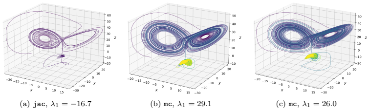
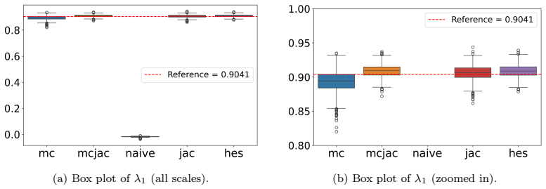
- In Lorenz 63, second-order supervision eliminates catastrophic Lyapunov-exponent outliers that appear under first-order methods with minimal temporal data.
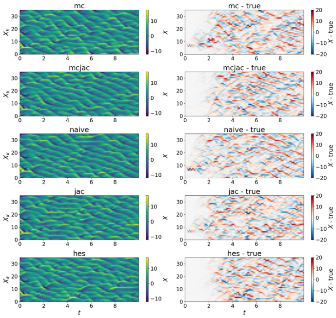
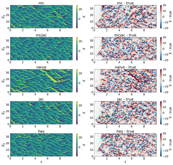
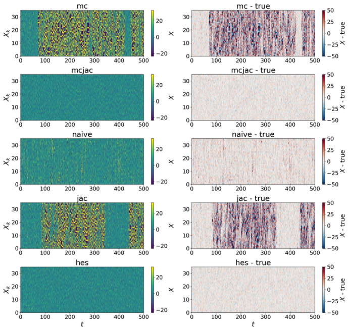
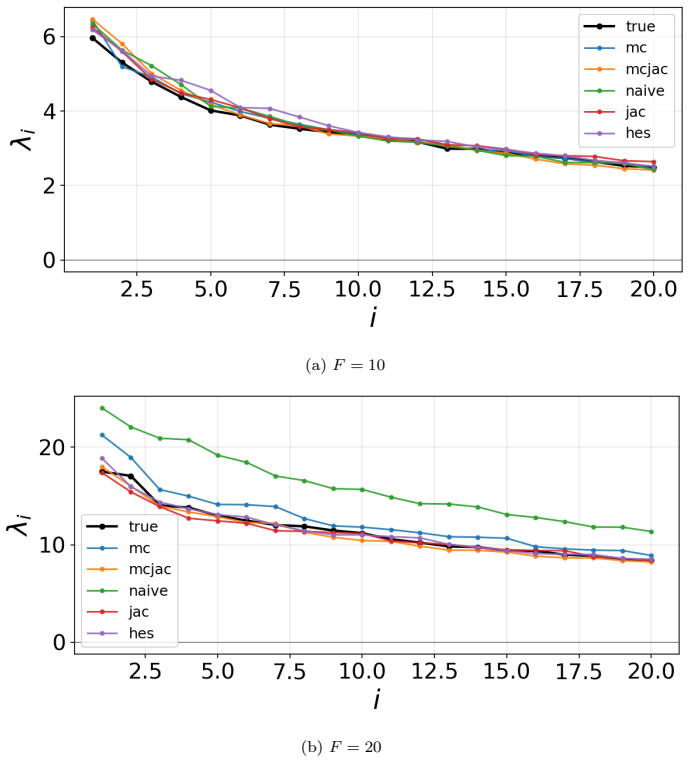
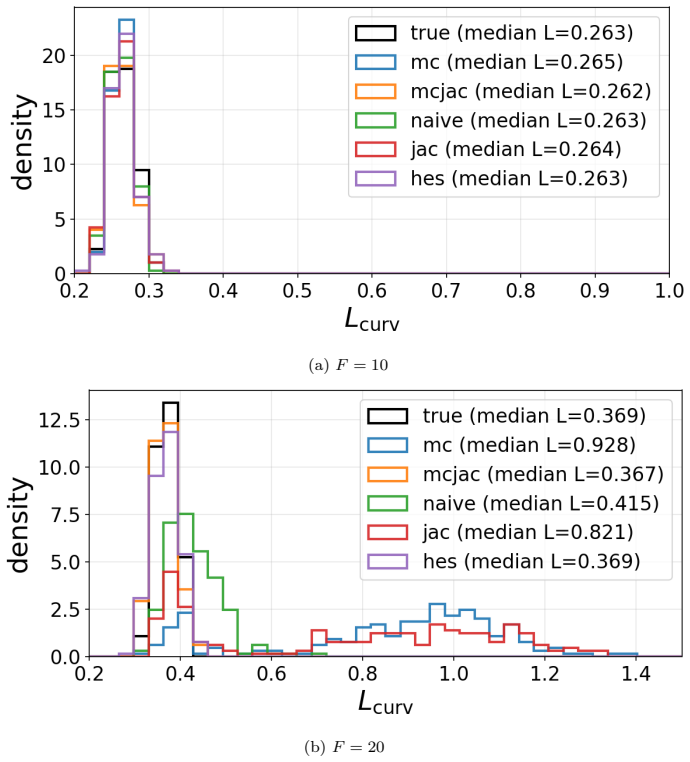
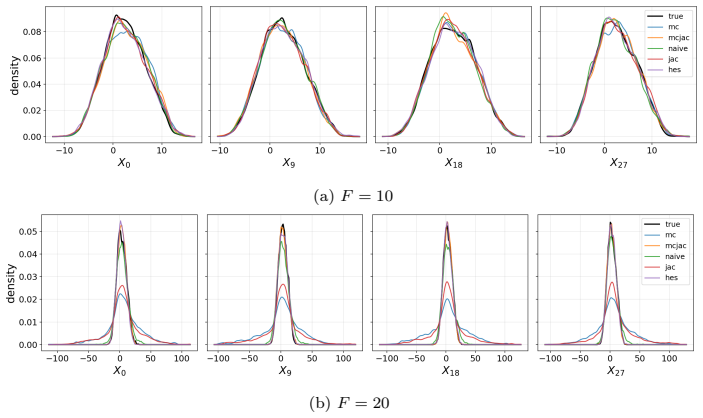
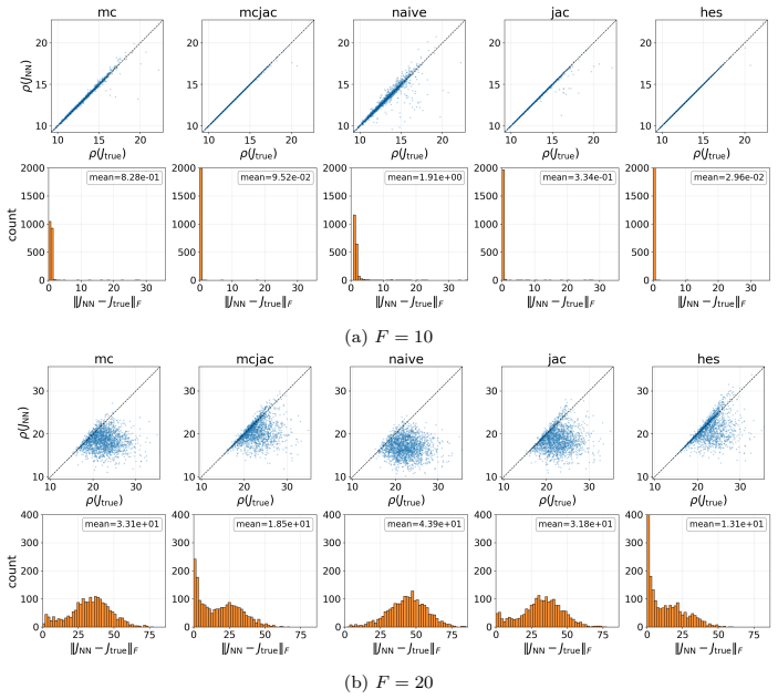
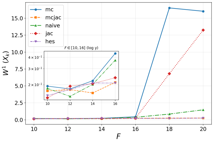
- In coupled Lorenz 96, second-order methods preserve the invariant measure and Lyapunov spectrum at forcing values beyond F=18 where first-order methods diverge.
- The randomized approach achieves performance comparable to explicit Hessian matching while remaining feasible in high dimensions.
- Only Jacobian evaluations are required, avoiding the prohibitive cost of forming the full Hessian tensor.
Where Pith is reading between the lines
- The same randomized-loss construction could be tested on other high-dimensional systems where explicit curvature information is unavailable but model evaluations remain cheap.
- If the perturbation variance must be tuned per system, the method may require an additional validation step not described in the core argument.
- The approach assumes the learned model remains queryable at arbitrary off-trajectory points, which may restrict its use when the model is defined only on observed data.
Load-bearing premise
The Taylor expansion of the vector field around the nominal point accurately captures the second-order contribution for the chosen perturbation variance.
What would settle it
A numerical verification that the difference in randomized Jacobian loss between two models exactly matches the predicted Hessian-mismatch term when Jacobian mismatch is held fixed and perturbation variance is varied.
Figures
read the original abstract
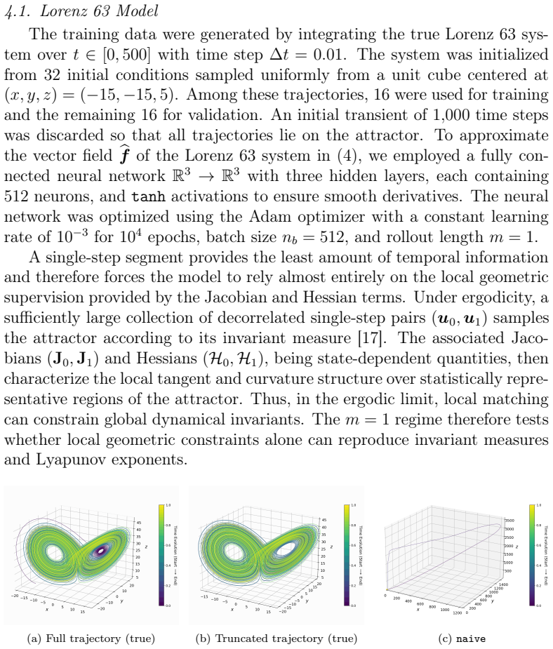
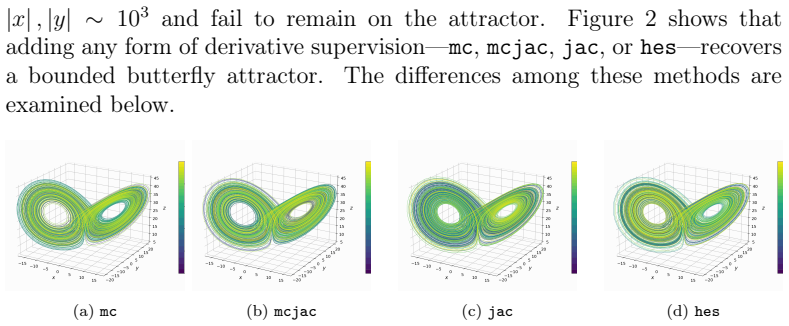
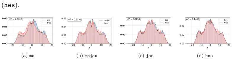
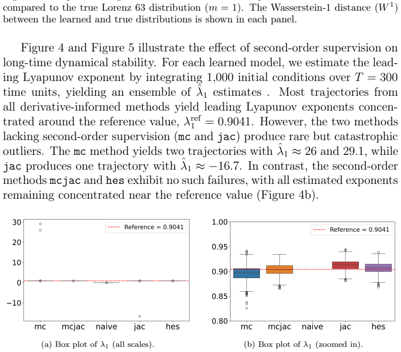
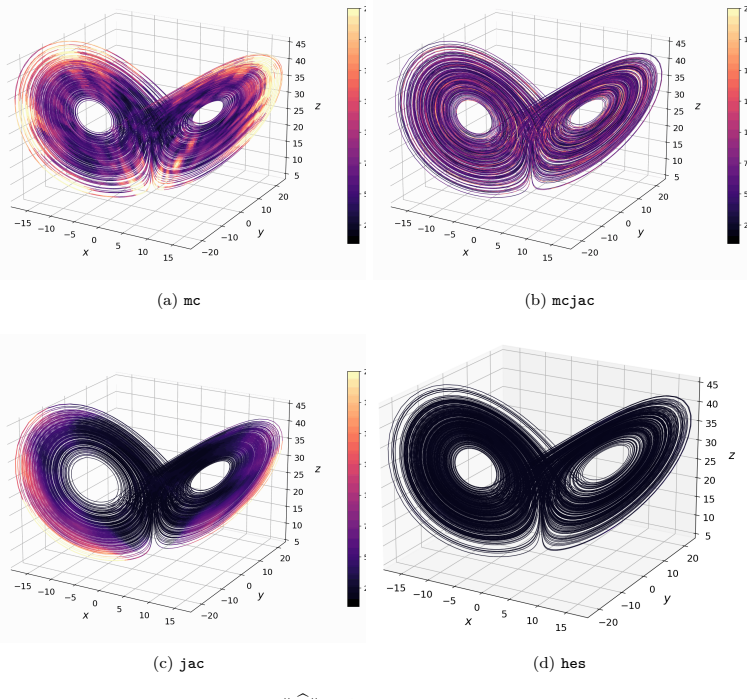
Learning chaotic dynamical systems from data requires more than short-term predictive accuracy: the learned model must preserve the attractor geometry and its invariant statistics. Trajectory (zero-order) and Jacobian (first-order) matching supervise the values and tangent structure of the vector field, but neither constrains how the field bends away from its tangent plane. A model can thus match values and tangents at the supervised states yet curve differently from the truth, remaining locally accurate while drifting toward spurious attractors and distorting long-time statistics. We show that enforcing second-order consistency mitigates these failures, but forming the full Hessian is prohibitive in high dimensions. We propose model-constrained randomized Jacobian matching, which compares the Jacobians of the true and learned vector fields at randomly perturbed inputs. A Taylor expansion shows that the expected randomized Jacobian loss decomposes into the nominal Jacobian mismatch plus a Hessian mismatch scaled by the noise variance, implicitly enforcing second-order consistency at $\mathcal{O}(d^2)$ cost without forming the $\mathcal{O}(d^3)$ Hessian tensor. Using only Jacobian evaluations, the method scales to high dimensions where explicit Hessian matching does not. Numerical experiments confirm that second-order methods are robust. For Lorenz~63, first-order methods produce catastrophic Lyapunov-exponent outliers under minimal temporal supervision, which second-order methods eliminate while recovering the correct attractor. For coupled Lorenz~96, an out-of-distribution forcing sweep separates the methods: all agree up to $F=16$, but beyond $F=18$ only second-order methods preserve the invariant measure and Lyapunov spectrum. On both systems, randomized Jacobian matching performs comparably to explicit Hessian matching at much lower cost.
Editorial analysis
A structured set of objections, weighed in public.
Referee Report
Summary. The manuscript proposes model-constrained randomized Jacobian matching as a way to enforce second-order geometric consistency when learning chaotic vector fields from data. A Taylor expansion of the Jacobian under random perturbations is used to show that the expected loss decomposes into the nominal first-order Jacobian mismatch plus a term proportional to the squared Hessian mismatch scaled by perturbation variance, achieving this supervision at O(d^2) cost without explicitly forming the O(d^3) Hessian. Experiments on Lorenz 63 and Lorenz 96 demonstrate that the approach eliminates failures of first-order methods (catastrophic Lyapunov outliers under minimal supervision; loss of invariant measure under out-of-distribution forcing) while matching the performance of explicit Hessian matching at lower cost.
Significance. If the central claim holds, the work supplies a practical, scalable route to second-order supervision for data-driven modeling of chaotic dynamics, where preservation of attractor geometry and long-time statistics is essential. The explicit Taylor decomposition, the exactness result for quadratic fields, and the reproducible numerical comparisons on standard benchmarks are strengths that strengthen the contribution.
major comments (2)
- [Abstract] Abstract and derivation of the randomized loss: the Taylor expansion is exact (remainder zero) only when third- and higher-order derivatives vanish, as occurs for the quadratic Lorenz systems in the experiments; for general C^3 fields the remainder term must be bounded or shown negligible for the chosen perturbation variance, otherwise the implicit second-order enforcement is not guaranteed.
- [Numerical experiments] Numerical experiments on Lorenz 96 (out-of-distribution forcing sweep): the separation of methods for F>18 is reported for the invariant measure and Lyapunov spectrum, but the manuscript must specify the number of Monte Carlo samples used to estimate the randomized loss, the perturbation variance schedule, and whether the reported differences are statistically significant across independent trials.
minor comments (2)
- The notation for the perturbation variance (denoted ε or σ in different places) should be unified and its scaling with dimension d discussed explicitly.
- A short paragraph on the computational complexity of Jacobian-vector products versus full Jacobian evaluations would clarify the claimed O(d^2) advantage.
Simulated Author's Rebuttal
We thank the referee for the positive assessment and constructive comments. We address each major comment below.
read point-by-point responses
-
Referee: [Abstract] Abstract and derivation of the randomized loss: the Taylor expansion is exact (remainder zero) only when third- and higher-order derivatives vanish, as occurs for the quadratic Lorenz systems in the experiments; for general C^3 fields the remainder term must be bounded or shown negligible for the chosen perturbation variance, otherwise the implicit second-order enforcement is not guaranteed.
Authors: We agree that the Taylor expansion of the Jacobian is exact (remainder zero) only for quadratic fields. The derivation isolates the leading Hessian term in the expectation under random perturbations, which holds exactly for the quadratic Lorenz systems used throughout the experiments. For general C^3 vector fields a remainder involving third derivatives scaled by the cube of the perturbation size appears. We will revise the manuscript to state this limitation explicitly, note that sufficiently small perturbation variance renders the remainder negligible relative to the O(σ^{2}) Hessian contribution, and add a brief remark on how the variance is chosen in practice to maintain this regime. revision: yes
-
Referee: [Numerical experiments] Numerical experiments on Lorenz 96 (out-of-distribution forcing sweep): the separation of methods for F>18 is reported for the invariant measure and Lyapunov spectrum, but the manuscript must specify the number of Monte Carlo samples used to estimate the randomized loss, the perturbation variance schedule, and whether the reported differences are statistically significant across independent trials.
Authors: We will revise the numerical-experiments section to report the exact number of Monte Carlo samples used to estimate the randomized Jacobian loss, the perturbation-variance schedule, and the outcome of statistical-significance tests (e.g., standard errors or p-values) computed across independent random seeds to substantiate the separation observed for F>18. revision: yes
Circularity Check
No significant circularity; derivation relies on external Taylor theorem
full rationale
The paper's central derivation applies the standard Taylor expansion to the randomized Jacobian loss, decomposing it into nominal Jacobian mismatch plus a scaled Hessian term. This is a direct mathematical identity from calculus, not dependent on any fitted parameters, self-referential definitions, or prior results by the same authors. No load-bearing step reduces to the paper's own inputs by construction, and the method's scaling advantage is computational rather than tautological. The experimental systems being quadratic makes the expansion exact but does not create circularity in the claim itself.
Axiom & Free-Parameter Ledger
axioms (1)
- standard math Taylor theorem applies to the vector field and its Jacobian under small perturbations
Reference graph
Works this paper leans on
-
[1]
J. P. Crutchfield, B. McNamara, Equations of motion from a data series, Complex Systems 1 (1987) 417–452. 34 Table A.7: Hyperparameters for the Lorenz 63 experiments (m= 1,2). Methodα mc αmcjac αjac αhes σlearning rate mc100– – –1.0 1×10 −3 mcjac100 100– –0.5 1×10 −3 naive– – – – –1×10 −3 jac– –1.0– –1×10 −3 hes– –1.0 0.1–1×10 −3 Table A.8: Hyperparameter...
1987
-
[2]
Kantz, T
H. Kantz, T. Schreiber, Nonlinear time series analysis, Cambridge Uni- versity Press, 2003
2003
-
[3]
S. L. Brunton, J. L. Proctor, J. N. Kutz, Discovering governing equa- tions from data by sparse identification of nonlinear dynamical systems, Proceedings of the National Academy of Sciences 113 (2016) 3932–3937
2016
-
[4]
R. T. Chen, Y. Rubanova, J. Bettencourt, D. K. Duvenaud, Neural ordi- nary differential equations, Advances in Neural Information Processing Systems 31 (2018)
2018
-
[5]
G. E. Karniadakis, I. G. Kevrekidis, L. Lu, P. Perdikaris, S. Wang, L. Yang, Physics-informed machine learning, Nature Reviews Physics 3 (2021) 422–440
2021
-
[6]
Raissi, P
M. Raissi, P. Perdikaris, G. E. Karniadakis, Physics-informed neural networks: A deep learning framework for solving forward and inverse problems involving nonlinear partial differential equations, Journal of Computational Physics 378 (2019) 686–707. 35
2019
-
[7]
P. R. Vlachas, W. Byeon, Z. Y. Wan, T. P. Sapsis, P. Koumoutsakos, Data-driven forecasting of high-dimensional chaotic systems with long short-termmemorynetworks, ProceedingsoftheRoyalSocietyA:Math- ematical, Physical and Engineering Sciences 474 (2018)
2018
-
[8]
J. Park, N. Yang, N. Chandramoorthy, When are dynamical systems learned from time series data statistically accurate?, Advances in Neural Information Processing Systems 37 (2024) 43975–44008
2024
-
[9]
X. Tian, Jacobian-Enforced neural networks (JENN) for improved data assimilation consistency in dynamical models, arXiv preprint arXiv:2412.01013 (2024)
-
[10]
Mohammadian, K
M. Mohammadian, K. Baker, F. Fioretto, Gradient-enhanced physics- informed neural networks for power systems operational support, Elec- tric Power Systems Research 223 (2023) 109551
2023
-
[11]
S. Zagoruyko, N. Komodakis, Paying more attention to attention: Im- proving the performance of convolutional neural networks via attention transfer, arXiv preprint arXiv:1612.03928 (2016)
work page internal anchor Pith review Pith/arXiv arXiv 2016
-
[12]
Srinivas, F
S. Srinivas, F. Fleuret, Knowledge transfer with Jacobian matching, in: International Conference on Machine Learning, PMLR, 2018, pp. 4723–4731
2018
-
[13]
Van Nguyen, J.-U
H. Van Nguyen, J.-U. Chen, T. Bui-Thanh, A model-constrained dis- continuous Galerkin network (DGNet) for compressible Euler equations with out-of-distribution generalization, Computer Methods in Applied Mechanics and Engineering 440 (2025) 117912
2025
-
[14]
H. V. Nguyen, T. Bui-Thanh, A model-constrained tangent slope learn- ing approach for dynamical systems, International Journal of Compu- tational Fluid Dynamics 36 (2022) 655–685
2022
-
[15]
E. N. Lorenz, Deterministic nonperiodic flow, Journal of Atmospheric Science 20 (1963) 130–141
1963
-
[16]
E.N.Lorenz, Predictability: Aproblempartlysolved, in: Proc.Seminar on Predictability, volume 1, Reading, 1996, pp. 1–18. 36
1996
-
[17]
Eckmann, D
J.-P. Eckmann, D. Ruelle, Ergodic theory of chaos and strange attrac- tors, Reviews of Modern Physics 57 (1985) 617
1985
-
[18]
Rüschendorf, The Wasserstein distance and approximation theorems, Probability Theory and Related Fields 70 (1985) 117–129
L. Rüschendorf, The Wasserstein distance and approximation theorems, Probability Theory and Related Fields 70 (1985) 117–129
1985
-
[19]
Villani, et al., Optimal transport: old and new, volume 338, Springer, 2009
C. Villani, et al., Optimal transport: old and new, volume 338, Springer, 2009
2009
-
[20]
Carlu, F
M. Carlu, F. Ginelli, V. Lucarini, A. Politi, Lyapunov analysis of mul- tiscale dynamics: the slow bundle of the two-scale Lorenz 96 model, Nonlinear Processes in Geophysics 26 (2019) 73–89
2019
-
[21]
J. C. Sprott, Chaos and time-series analysis, Oxford University Press, 2003
2003
-
[22]
Benettin, L
G. Benettin, L. Galgani, A. Giorgilli, J.-M. Strelcyn, Lyapunov char- acteristic exponents for smooth dynamical systems and for Hamiltonian systems; a method for computing all of them. Part 1: Theory, Meccanica 15 (1980) 9–20
1980
-
[23]
Universal Differential Equations for Scientific Machine Learning
C. Rackauckas, Y. Ma, J. Martensen, C. Warner, K. Zubov, R. Supekar, D. Skinner, A. Ramadhan, A. Edelman, Universal differential equations for scientific machine learning, arXiv preprint arXiv:2001.04385 (2020)
work page internal anchor Pith review Pith/arXiv arXiv 2001
-
[24]
Tsitouras, Runge–Kutta pairs of order 5 (4) satisfying only the first column simplifying assumption, Computers & Mathematics with Appli- cations 62 (2011) 770–775
C. Tsitouras, Runge–Kutta pairs of order 5 (4) satisfying only the first column simplifying assumption, Computers & Mathematics with Appli- cations 62 (2011) 770–775. 37
2011
discussion (0)
Sign in with ORCID, Apple, or X to comment. Anyone can read and Pith papers without signing in.