A Preliminary Model for Managing Technical Debt in an Agile Environment
Pith reviewed 2026-06-27 20:57 UTC · model grok-4.3
The pith
A dynamic policy balances new agile development against technical debt remediation by weighing current economic value against future velocity gains.
A machine-rendered reading of the paper's core claim, the machinery that carries it, and where it could break.
Core claim
The model distinguishes initiated but unfinished functional debt from defects and rework, interprets velocity decline as debt interest, derives the limitations of a naive maximum-remediation rule, and replaces it with a dynamic allocation policy uk that incorporates decreasing marginal value; when applied to discrete inhomogeneous items the policy produces simulation trajectories consistent with the economic premise that sometimes allowing debt to grow is value-superior to immediate repayment.
What carries the argument
The dynamic policy uk, which at each step chooses the fraction of velocity allocated to remediation versus new development on the basis of current debt stock, marginal story value and intertemporal value comparison.
If this is right
- A team following uk will sometimes deliberately defer remediation and still finish with higher total value than a team that always clears debt first.
- Productivity loss can be expressed as an explicit interest rate on the existing debt stock.
- The same decision rule remains well-defined when stories differ in size and value and when only a macroscopic view of the backlog is available.
- Sensitivity checks confirm that the qualitative behaviour survives reasonable variation in the model parameters.
- The formulation is limited to settings where organisational parameters remain stable across the planning horizon.
Where Pith is reading between the lines
- The policy could be embedded in an automated backlog prioritisation tool that re-computes uk each sprint from measured velocity and story estimates.
- Real project data on velocity degradation versus debt size would allow calibration of the marginal-value curve that the model leaves as a free parameter.
- If story coupling proves stronger than assumed, the macroscopic policy would need an explicit interaction term before deployment.
Load-bearing premise
The model requires that decision makers can accurately compare present and future economic value and that individual stories interact only weakly so their ordering effects can be ignored.
What would settle it
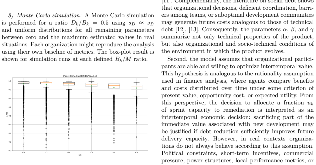
Running the Monte Carlo simulation with the uk policy turned off (i.e., forcing either zero or full remediation each period) and observing whether total cumulative value across the horizon falls below the value obtained when uk is active would directly test the claimed superiority.
Figures
read the original abstract
This paper presents a preliminary model for managing involuntary technical debt in agile environments by formulating, in an integrated way, the dynamics among backlog, debt, velocity, and economic value. The work distinguishes initiated but unfinished functional debt from a simple defect back log and from rework, interprets productivity degradation as technical-debt interest, and derives the naive maximum-remediation policy in order to show its limitations against an intertemporal value-based decision. On this basis, a dynamic policy uk is proposed to balance new development and remediation; a decreasing marginal-value structure is incorporated; and the model is extended to discrete, inhomogeneous items. Exploratory validation through sensitivity analysis and MonteCarlo simulation shows behavior consistent with the economic intuition of the model. Finally, the limits of the formulation are made explicit: its macroscopic nature, its dependence on organizationally stable parameters, its assumption of intertemporal rationality, and its requirement of weak coupling among stories.
Editorial analysis
A structured set of objections, weighed in public.
Referee Report
Summary. This paper presents a preliminary model for managing involuntary technical debt in agile environments by formulating the dynamics among backlog, debt, velocity, and economic value. It distinguishes initiated but unfinished functional debt from defect backlog and rework, interprets productivity degradation as technical-debt interest, derives the naive maximum-remediation policy to show its limitations against an intertemporal value-based decision, proposes a dynamic policy uk to balance new development and remediation with a decreasing marginal-value structure, extends the model to discrete inhomogeneous items, and reports exploratory validation via sensitivity analysis and Monte Carlo simulation showing behavior consistent with economic intuition. The formulation's limits (macroscopic scale, organizationally stable parameters, intertemporal rationality, weak coupling) are explicitly stated.
Significance. If the result holds, the integrated model offers a structured economic-value approach to technical debt decisions in agile settings, with the dynamic policy uk and discrete-item extension providing a basis for balancing remediation against new development. The explicit listing of limits and the use of simulation to confirm internal consistency with intuition are strengths for a preliminary formulation; however, the absence of external benchmarks or independent parameter grounding limits immediate practical impact.
major comments (2)
- [dynamic policy uk section] The derivation of the dynamic policy uk relies on the model's equations for economic value and velocity degradation (treated as interest) that are defined in terms of organizationally stable parameters; this dependence is load-bearing for the claim that uk provides a balanced, value-based alternative to the naive policy, yet the parameters lack independent grounding outside the formulation.
- [exploratory validation section] The Monte Carlo simulation and sensitivity analysis are presented as showing consistency with economic intuition for the discrete inhomogeneous extension, but without reported error bounds, convergence diagnostics, or external data benchmarks this validation remains internal and does not independently test the weak-coupling assumption that underpins the discrete-item claim.
minor comments (2)
- The abstract opens with a long compound sentence; splitting the core contribution (formulation of uk plus discrete extension) into a clearer lead sentence would improve readability.
- Notation uk for the dynamic policy should be introduced with an explicit definition on first appearance rather than assumed from context.
Simulated Author's Rebuttal
We thank the referee for the constructive comments and the recommendation of minor revision. We address each major comment below.
read point-by-point responses
-
Referee: [dynamic policy uk section] The derivation of the dynamic policy uk relies on the model's equations for economic value and velocity degradation (treated as interest) that are defined in terms of organizationally stable parameters; this dependence is load-bearing for the claim that uk provides a balanced, value-based alternative to the naive policy, yet the parameters lack independent grounding outside the formulation.
Authors: We agree that the parameters lack independent empirical grounding and are treated as organizationally stable by assumption; this is explicitly listed as a limit of the formulation. The dynamic policy uk is derived within the stated scope of the preliminary model to show an intertemporal value-based alternative to the naive maximum-remediation policy. No external grounding is claimed or possible in this theoretical work. We will add a brief clarifying sentence in the dynamic policy section to restate the scope. revision: partial
-
Referee: [exploratory validation section] The Monte Carlo simulation and sensitivity analysis are presented as showing consistency with economic intuition for the discrete inhomogeneous extension, but without reported error bounds, convergence diagnostics, or external data benchmarks this validation remains internal and does not independently test the weak-coupling assumption that underpins the discrete-item claim.
Authors: The validation is described as exploratory and is intended only to confirm internal consistency with economic intuition, not to test assumptions such as weak coupling (which is stated as a model limit) or to provide external benchmarks. We acknowledge the lack of reported error bounds and convergence diagnostics. We will revise the validation section to include these diagnostics while preserving the exploratory framing. revision: yes
Circularity Check
No significant circularity detected
full rationale
The paper formulates a model from explicit assumptions on backlog dynamics, velocity degradation interpreted as interest, and intertemporal value, then proposes a dynamic policy uk and discrete extension on that basis. Validation consists of sensitivity analysis and Monte Carlo runs that reproduce the model's own economic intuition, which is expected behavior for an internally consistent formulation rather than a reduction of outputs to inputs by construction. No equations are shown to define a quantity in terms of itself, no fitted parameters are relabeled as predictions, and no self-citations serve as load-bearing justification for uniqueness or ansatzes. The work is self-contained within its stated macroscopic scope and limits, with no load-bearing step reducing to its own inputs.
Axiom & Free-Parameter Ledger
free parameters (2)
- organizationally stable parameters
- marginal value parameters
axioms (2)
- domain assumption intertemporal rationality of decision makers
- domain assumption weak coupling among stories
invented entities (1)
-
dynamic policy uk
no independent evidence
Reference graph
Works this paper leans on
-
[1]
The WyCash Portfolio Management Sys- tem,
W. Cunningham, “The WyCash Portfolio Management Sys- tem,” inOOPSLA Experience Report, 1992
1992
-
[2]
Technical Debt,
S. McConnell, “Technical Debt,”IEEE Software, vol. 25, no. 6, pp. 103–104, 2008
2008
-
[3]
Technical Debt: From Metaphor to Theory and Practice,
P. Kruchten, R. L. Nord, and I. Ozkaya, “Technical Debt: From Metaphor to Theory and Practice,”IEEE Software, vol. 29, no. 6, pp. 18–21, 2012
2012
-
[4]
Kruchten, R
P. Kruchten, R. L. Nord, and I. Ozkaya,Managing Technical Debt: Reducing Friction in Software Development. Boston, MA, USA: Addison-Wesley, 2019
2019
-
[5]
Managing Technical Debt in Software-Reliant Systems,
N. Brown, Y. Cai, Y. Guo, R. Kazman, M. Kim, P. Kruchten, E. Lim, A. MacCormack, R. Nord, I. Ozkaya, R. Sangwan, C. Sea- man, K. Sullivan, and N. Zazworka, “Managing Technical Debt in Software-Reliant Systems,” inProceedings of the FSE/SDP Workshop on Future of Software Engineering Research, pp. 47– 52, 2010
2010
-
[6]
Using Analytics to Quantify the Interest of Self-Admitted Technical Debt,
Y. Kamei, E. Maldonado, E. Shihab, and N. Ubayashi, “Using Analytics to Quantify the Interest of Self-Admitted Technical Debt,” inProceedings of the Third International Workshop on Technical Debt Analytics (TDA) , CEUR Workshop Proceed- ings, vol. 1771, pp. 68–71, 2016
2016
-
[7]
Establishing a Framework for Managing Interest in Technical Debt,
A. Ampatzoglou, A. Ampatzoglou, P. Avgeriou, and A. Chatzi- georgiou, “Establishing a Framework for Managing Interest in Technical Debt,” inProceedings of the 5th International Sympo- sium on Business Modeling and Software Design (BMSD) , pp. 75–85, 2015
2015
-
[8]
On the Interest of Architectural Tech- nical Debt: Uncovering the Contagious Debt Phenomenon,
A. Martini and J. Bosch, “On the Interest of Architectural Tech- nical Debt: Uncovering the Contagious Debt Phenomenon,” Journal of Software: Evolution and Process, vol. 29, no. 10, Art. e1877, 2017
2017
-
[9]
A Large-Scale Empirical Study on Self-Admitted Technical Debt,
G. Bavota and B. Russo, “A Large-Scale Empirical Study on Self-Admitted Technical Debt,” inProceedings of the 13th Inter- national Conference on Mining Software Repositories (MSR) , pp. 315–326, 2016
2016
-
[10]
InvestigatingArchitec- tural Technical Debt Accumulation and Refactoring over Time: A Multiple-Case Study,
A.Martini,J.Bosch,andM.Chaudron,“InvestigatingArchitec- tural Technical Debt Accumulation and Refactoring over Time: A Multiple-Case Study,”Information and Software Technology, vol. 67, pp. 237–253, 2015
2015
-
[11]
Socio-Technical Congruence:AFrameworkforAssessingtheImpactofTechnical and Work Dependencies on Software Development Productiv- ity,
M. Cataldo, J. D. Herbsleb, and K. M. Carley, “Socio-Technical Congruence:AFrameworkforAssessingtheImpactofTechnical and Work Dependencies on Software Development Productiv- ity,” inProceedings of the Second ACM-IEEE International Symposium on Empirical Software Engineering and Measure- ment (ESEM), pp. 2–11, 2008
2008
-
[12]
What Is Social Debt in Software Engineering?
D. A. Tamburri, P. Kruchten, P. Lago, and H. van Vliet, “What Is Social Debt in Software Engineering?” inProceedings of the 6th International Workshop on Cooperative and Human Aspects of Software Engineering (CHASE) , pp. 93–96, 2013
2013
-
[13]
Social Debt in Software Engineering: Insights from Industry,
D. A. Tamburri, P. Kruchten, P. Lago, and H. van Vliet, “Social Debt in Software Engineering: Insights from Industry,”Journal of Internet Services and Applications , vol. 6, no. 1, 2015
2015
-
[14]
Reinertsen, The Principles of Product Development Flow: Second Generation Lean Product Development
D. Reinertsen, The Principles of Product Development Flow: Second Generation Lean Product Development. Redondo Beach, CA, USA: Celeritas, 2009
2009
-
[15]
Damodaran, Investment Valuation: Tools and Techniques for Determining the Value of Any Asset,3rded.Hoboken,NJ,USA: Wiley, 2012
A. Damodaran, Investment Valuation: Tools and Techniques for Determining the Value of Any Asset,3rded.Hoboken,NJ,USA: Wiley, 2012
2012
-
[16]
Programs, Life Cycles, and Laws of Software Evolution,
M. M. Lehman, “Programs, Life Cycles, and Laws of Software Evolution,”Proceedings of the IEEE , vol. 68, no. 9, pp. 1060– 1076, 1980
1980
-
[17]
Distributed Agile, Agile Testing, and Technical Debt,
R. Bavani, “Distributed Agile, Agile Testing, and Technical Debt,”IEEE Software , vol. 29, no. 6, pp. 28–33, 2012, doi: 10.1109/MS.2012.155
-
[18]
Perfectionists in a World of Finite Resources,
F. Shull, “Perfectionists in a World of Finite Resources,”IEEE Software, vol. 28, no. 2, pp. 4–6, 2011, doi: 10.1109/MS.2011.38
-
[19]
Poppendieck and T
M. Poppendieck and T. Poppendieck,Lean Software Develop- ment: An Agile Toolkit, Addison-Wesley, 2003
2003
-
[20]
Cohn, Agile Estimating and Planning
M. Cohn, Agile Estimating and Planning . Upper Saddle River, NJ, USA: Prentice Hall, 2005
2005
-
[21]
Fowler,Refactoring: Improving the Design of Existing Code
M. Fowler,Refactoring: Improving the Design of Existing Code . Boston, MA, USA: Addison-Wesley, 1999
1999
-
[22]
Jones, Software Engineering Best Practices , McGraw-Hill, 2010
C. Jones, Software Engineering Best Practices , McGraw-Hill, 2010
2010
-
[23]
Mens and S
T. Mens and S. Demeyer,Software Evolution, Springer, 2008
2008
-
[24]
B. W. Boehm, Software Engineering Economics . Englewood Cliffs, NJ, USA: Prentice Hall, 1981
1981
-
[25]
Technical Debt in Practice: A Study on Software Development Projects,
H. Erdogmus, O. Sievi-Korte, and J. Järvi, “Technical Debt in Practice: A Study on Software Development Projects,”IEEE Software, 2016
2016
-
[26]
The Impact of Code Smells on Software Quality: A Study of Technical Debt,
I. Ahmed, B. Adams, and A. E. Hassan, “The Impact of Code Smells on Software Quality: A Study of Technical Debt,” Empirical Software Engineering, 2015. Appendix Appendix A: Estimation of V alue-Relationship Parameters The model assumes a value relationship in a prioritized backlog approximately characterized by a Pareto/Zipf dis- tribution. Let a sequence...
2015
-
[27]
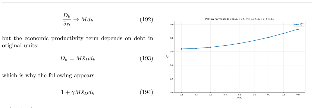
lnxn (A.15) X = 1 ln 1 1 ln 2
Estimation by linear regression: The estimation of the parameters is obtained by ordinary least squares: ˆb = ∑n k=1(zk−¯z)(yk−¯y)∑n k=1(zk−¯z)2 (A.9) ˆa = ¯y−ˆb¯z (A.10) where: ¯y = 1 n n∑ k=1 yk (A.11) ¯z = 1 n n∑ k=1 zk (A.12) The original parameters are recovered as: ˆα=−ˆb (A.13) ˆC =eˆa (A.14) The model can be written in matrix form as: y = l...
-
[28]
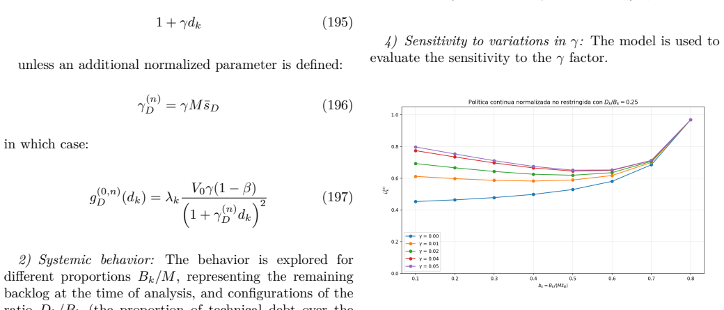
Bias of the logarithmic estimator:It should be noted that: E[lnx]̸= lnE[x] (A.18) which implies that log-log regression introduces bias in finite samples
-
[29]
Alternative estimation: maximum likelihood:Assum- ing a continuous Pareto distribution: f(x) =dxs minx−(s+1) (A.19) the maximum-likelihood estimator is: ˆα= [ 1 n n∑ i=1 ln xi xmin ]−1 (A.20)
-
[30]
Applying logarithms: lnxk = lnC−s ln(k +δ) (A.22) This model is not linear in the parameters and requires nonlinear least-squares estimation
Extension: truncated Zipf law:To improve the fit in real data, the following can be used: xk = C (k +δ)s (A.21) with δ >0. Applying logarithms: lnxk = lnC−s ln(k +δ) (A.22) This model is not linear in the parameters and requires nonlinear least-squares estimation
-
[31]
This directly impacts the optimal effort allocation in the main model
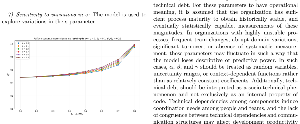
Interpretation in the technical-debt model:The pa- rameter αcharacterizes value concentration: •highs> 0 implies strong value concentration in a few items; •s≈1 corresponds to classic Zipf-like behavior; •s< 1 indicates a heavy tail and a more homogeneous distribution. This directly impacts the optimal effort allocation in the main model
-
[32]
In particular: s↑ ⇒ηk↓ (A.24) which connects the distribution of value with the opera- tional efficiency of the sprint
Relationship with packing efficiency: The hetero- geneity induced byαaffects sprint efficiency: ηk = 1−Wk Vk (A.23) where Wk represents unused capacity due to indivisibili- ties. In particular: s↑ ⇒ηk↓ (A.24) which connects the distribution of value with the opera- tional efficiency of the sprint. Appendix B: Empirical Estimation of the Degradation Parame...
-
[33]
Estimation under the exponential model: Starting from: Vk =V0e−γDk (B.4) Applying logarithms: lnVk = lnV0−γDk (B.5) Defining: yk = lnVk (B.6) xk =Dk (B.7) the linear model is obtained: yk =a +bxk +εk (B.8) where: a = lnV0 (B.9) b =−γ (B.10) The least-squares estimation is: ˆb = ∑n k=1(xk−¯x)(yk−¯y)∑n k=1(xk−¯x)2 (B.11) ˆa = ¯y−ˆb¯x (B.12) therefore: ˆγ=−ˆb (B.13)
-
[34]
Estimation under the rational model:Considering: Vk = V0 1 +γDk (B.14) it can be rewritten as: 1 Vk = 1 V0 + γ V0 Dk (B.15) Defining: yk = 1 Vk (B.16) xk =Dk (B.17) we obtain: yk =a +bxk (B.18) where: a = 1 V0 (B.19) b = γ V0 (B.20) Then: ˆγ= ˆb ˆa (B.21)
-
[35]
Direct nonlinear estimation:Alternatively,γmay be estimated by solving: min γ,V0 n∑ k=1 ( Vk−V0e−γDk )2 (B.22) or: min γ,V0 n∑ k=1 ( Vk− V0 1 +γDk )2 (B.23) This approach avoids transformations and reduces bias, but requires iterative methods. B. Parameter interpretation The parameterγcan be interpreted as: γ=−1 Vk ∂Vk ∂Dk (B.24) which represents the marg...
-
[36]
In particular: γ↑ ⇒u⋆ k↑ (B.25) which implies greater optimal allocation toward technical- debt reduction
Consistency with the discrete model:The estimation of γinfluences the optimal policyu⋆ k of the main model, because it affects the marginal valuation of reducing debt relative to producing backlog. In particular: γ↑ ⇒u⋆ k↑ (B.25) which implies greater optimal allocation toward technical- debt reduction. Appendix C: Characterization and Estimation of the E...
-
[37]
Performed under grant UADER FCyT Project PI-B 230/24 19
Relationship with productivity improvement:If a re- duction in technical debt produces an increase in future velocity ∆Vk, the increase in value can be approximated by: ∆νk≈λ∆Vk (C.2) which justifies the use ofλin equations (84) and (85) of the main model. Performed under grant UADER FCyT Project PI-B 230/24 19
-
[38]
Empirical model: To estimate λ, it is proposed to model the relationship between economic value and veloc- ity: νk =ν0 +λVk +εk (C.3) where: •νk: economic value generated in sprintk; •Vk: velocity (delivered story points); •ν0: base value independent of velocity; •εk: error term
-
[39]
Estimation by linear regression:Defining: yk =νk (C.4) xk =Vk (C.5) we obtain: yk =a +bxk +εk (C.6) where: a =ν0 (C.7) b =λ (C.8) The least-squares estimator is: ˆλ= ∑n k=1(xk−¯x)(yk−¯y)∑n k=1(xk−¯x)2 (C.9) with: ¯x = 1 n n∑ k=1 Vk (C.10) ¯y = 1 n n∑ k=1 νk (C.11)
-
[40]
Incremental estimation: To eliminate the base term ν0, a differences formulation can be used: ∆νk =νk−νk−1 (C.12) ∆Vk =Vk−Vk−1 (C.13) and fit: ∆νk =λ∆Vk +εk (C.14)
-
[41]
Required data:To estimateλ, the following dataset is required: {(Vk,νk)}n k=1 (C.15) where: •Vk: sprint velocity (completed story points); •νk: generated economic value. The valueνk can be approximated through: •revenue generated in the sprint; •business value assigned to completed stories; •story points weighted by relative value; •economic proxies deriv...
-
[42]
Economic interpretation: The parameter λrepre- sents: λ>0 (C.16) and its magnitude indicates the marginal value of capacity: •high λ: strong return from increasing velocity; •lowλ: decreasing returns
-
[43]
Nonlinear extension:If the relationship is not linear, one may consider: νk =f(Vk) (C.17) and define: λ= df(Vk) dVk (C.18) In this case, linear regression estimates an average value of λover the observed range
-
[44]
In particular: λ↑ ⇒u⋆ k↑ (C.19) which implies a greater incentive to invest in debt reduc- tion in order to improve future capacity
Consistency with the decision model:The value ofλ determines the economic benefit of increasing future veloc- ity, and therefore directly influences the optimal decision of effort allocation between backlog and technical debt. In particular: λ↑ ⇒u⋆ k↑ (C.19) which implies a greater incentive to invest in debt reduc- tion in order to improve future capacit...
discussion (0)
Sign in with ORCID, Apple, or X to comment. Anyone can read and Pith papers without signing in.