Kling-Gupta linear regression
Pith reviewed 2026-06-27 14:47 UTC · model grok-4.3
The pith
Kling-Gupta linear regression scales the ordinary least squares coefficient vector by a variance-inflation factor based on sample variances and covariances.
A machine-rendered reading of the paper's core claim, the machinery that carries it, and where it could break.
Core claim
Minimizing the negatively oriented Kling-Gupta loss L_KG = (1 - KGE)^2 in multiple linear regression produces coefficient estimates that scale the ordinary least squares vector by a variance-inflation factor governed by the sample variances and covariances of the predictors and response. The resulting predictions replicate the sample variance of the observations on the training set, while both the Kling-Gupta and ordinary least squares estimators match the sample mean of the observations and achieve identical sample correlations between predictions and observations. The Kling-Gupta estimator converges almost surely to well-defined population limits expressed algebraically in terms of the und
What carries the argument
The explicit scaling of the ordinary least squares coefficient vector by a variance-inflation factor determined by sample variances and covariances.
If this is right
- Kling-Gupta regression predictions exactly replicate the sample variance of the response on the training set.
- Both estimators match the sample mean of the observations and achieve the same sample correlation between predictions and observations.
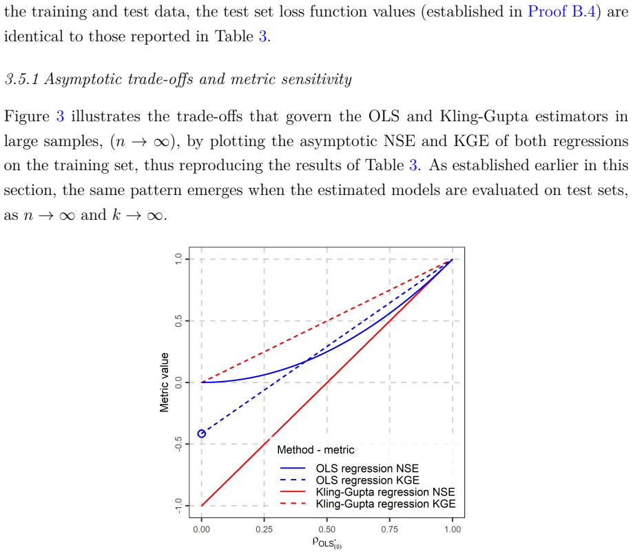
- The ordinary least squares estimator attains the maximum possible Nash-Sutcliffe efficiency but not the maximum Kling-Gupta efficiency, while the Kling-Gupta estimator does the reverse.
- The Kling-Gupta estimator converges almost surely to explicit algebraic population limits, and training and test performance metrics converge to identical asymptotic values.
Where Pith is reading between the lines
- In hydrology applications, fitting directly to the Kling-Gupta loss may produce models whose predictions better retain the variability seen in observed data.
- The demonstrated impossibility of jointly maximizing NSE and KGE creates a concrete trade-off that modelers must navigate when selecting a loss function.
- The scaling relation derived here could be tested for persistence when the Kling-Gupta loss is applied inside nonlinear or regularized regression frameworks.
Load-bearing premise
The negatively oriented Kling-Gupta loss can be directly minimized in a standard multiple linear regression model using the usual sample moments without additional constraints or modifications to the loss definition.
What would settle it
On any finite dataset compute the ordinary least squares coefficients, the sample variances and covariances, and the stated variance-inflation factor; if the Kling-Gupta coefficient estimates deviate from the predicted scaled vector then the explicit formulas are falsified.
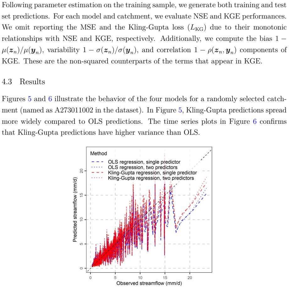
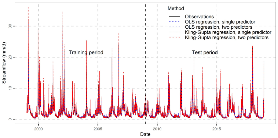
Figures

read the original abstract
Although the Kling-Gupta efficiency ($\mathrm{KGE}$) is widely adopted for model evaluation in hydrology, its properties as a statistical estimator remain unexplored. Investigating these properties is necessary because parameter estimation and forecast evaluation are inherently linked. To address this, we formalize the negatively oriented Kling-Gupta loss $L_\mathrm{KG} = (1 - \mathrm{KGE})^2$ within an extremum estimation framework (equivalent to maximizing $\mathrm{KGE}$) and analyze its behavior in multiple linear regression. We establish explicit formulas for the parameter estimates, showing that Kling-Gupta linear regression scales the ordinary least squares (OLS) coefficient vector by a variance-inflation factor governed by the sample variances and covariances of the predictors and the response. We show that Kling-Gupta linear regression predictions replicate the sample variance of the response on the training set, in contrast to the variance reduction inherent to OLS, while both estimators maintain the sample mean of the observations and achieve the same sample correlation between the predictions and the response. We show analytically that no single estimator can simultaneously maximize both the Nash-Sutcliffe efficiency $\mathrm{NSE}$ and $\mathrm{KGE}$: the OLS estimator attains the maximum possible $\mathrm{NSE}$ but not the maximum $\mathrm{KGE}$, while the Kling-Gupta estimator maximizes $\mathrm{KGE}$ at the cost of $\mathrm{NSE}$. We prove the almost sure convergence of the Kling-Gupta estimator to well-defined population limits and express those limits algebraically. Furthermore, we evaluate the training and test set performance metrics for both estimators, demonstrating that for each estimator the metrics on the training set and on an independent test set converge asymptotically to identical limits (though the limits differ between OLS and Kling-Gupta regression).
Editorial analysis
A structured set of objections, weighed in public.
Referee Report
Summary. The paper formalizes the negatively oriented Kling-Gupta loss L_KG = (1 - KGE)^2 within an extremum estimation framework for multiple linear regression. It derives explicit algebraic formulas for the parameter estimates, showing that the Kling-Gupta estimator scales the OLS coefficient vector by a variance-inflation factor based on sample variances and covariances. The resulting predictions match the sample variance of the response (unlike OLS), while both estimators match the sample mean and achieve identical sample correlation with the response. The paper proves that no single estimator can simultaneously maximize NSE and KGE, establishes almost-sure convergence of the Kling-Gupta estimator and its metrics to explicit population limits via the LLN, and shows that training and test metrics converge to the same asymptotic limits (differing between the two estimators).
Significance. If the central derivations hold, the manuscript supplies explicit closed-form expressions, a variance-matching property, an NSE-KGE incompatibility result, and LLN-based convergence statements for KGE-based regression. These algebraic characterizations and the explicit population limits constitute clear strengths for a statistics paper, providing a precise link between a widely used hydrological metric and standard regression estimators.
minor comments (2)
- [§3] §3: the variance-inflation factor is described in the text but would benefit from an explicit numbered equation to facilitate cross-reference with the population-limit expressions later in the paper.
- [Notation] Notation section: sample moments and population quantities are used throughout; a brief table or sentence distinguishing the two (e.g., r vs. ρ) would improve readability of the convergence statements.
Simulated Author's Rebuttal
We thank the referee for the positive and accurate summary of the manuscript, the recognition of its algebraic characterizations and population limits as strengths, and the recommendation for minor revision. We are pleased that the central results on the Kling-Gupta estimator, its variance-matching property, the NSE-KGE incompatibility, and the LLN convergence are viewed favorably.
Circularity Check
No significant circularity; derivation is self-contained
full rationale
The paper starts from the explicit definition of the negatively oriented KGE loss L_KG = (1 - KGE)^2 and standard sample moments (means, variances, covariances, correlation) within an extremum estimation framework for multiple linear regression. It derives the closed-form estimator as a scaled OLS coefficient vector by maximizing correlation subject to the variance-matching constraint that is built into KGE, then applies the LLN to obtain population limits expressed algebraically in the same moments. These steps rely only on the algebraic properties of sample correlation and variance plus standard convergence arguments; no parameter is fitted to a subset and then renamed as a prediction, no self-citation supplies a uniqueness theorem, and no ansatz is smuggled in. The incompatibility between NSE and KGE maximizers follows directly from the differing objective functions. The analysis is therefore independent of its inputs and receives the default non-circularity finding.
Axiom & Free-Parameter Ledger
axioms (2)
- standard math Sample variances and covariances exist and the predictor matrix permits the usual OLS inversion
- domain assumption KGE is composed of its three standard components (correlation, bias ratio, variability ratio) as defined in the hydrology literature
Reference graph
Works this paper leans on
-
[1]
Allaire JJ, Xie Y, Dervieux C, McPherson J, Luraschi J, Ushey K, Atkins A, Wickham H, Cheng J, Chang W, Iannone R (2026) rmarkdown: Dynamic Documents for R. R package version 2.31. https://doi.org/10.32614/CRAN.package.rmarkdown
-
[2]
Amemiya T (1973) Regression analysis when the dependent variable is truncated normal. Econometrica 41(6): 997--1016 . https://doi.org/10.2307/1914031
-
[3]
Cambridge, MA: Harvard University Press
Amemiya T (1985) Advanced Econometrics. Cambridge, MA: Harvard University Press. ISBN: 9780674251991
1985
-
[4]
Chemometrics and Intelligent Laboratory Systems 33(1): 17--33
Amrhein M, Srinivasan B, Bonvin D, Schumacher MM (1996) On the rank deficiency and rank augmentation of the spectral measurement matrix. Chemometrics and Intelligent Laboratory Systems 33(1): 17--33 . https://doi.org/10.1016/0169-7439(95)00086-0
-
[5]
IEEE Transactions on Information Theory 51(7): 2664--2669
Banerjee A, Guo X, Wang H (2005) On the optimality of conditional expectation as a Bregman predictor. IEEE Transactions on Information Theory 51(7): 2664--2669 . https://doi.org/10.1109/TIT.2005.850145
-
[6]
Barrett T, Dowle M, Srinivasan A, Gorecki J, Chirico M, Hocking T, Schwendinger B, Krylov I (2026) data.table: Extension of 'data.frame'. R package version 1.18.4. https://doi.org/10.32614/CRAN.package.data.table
-
[7]
Environmental Modelling and Software 40: 1--20
Bennett ND, Croke BFW, Guariso G, Guillaume JHA, Hamilton SH, Jakeman AJ, Marsili-Libelli S, Newham LTH, Norton JP, Perrin C, Pierce SA, Robson B, Seppelt R, Voinov AA, Fath BD, Andreassian V (2013) Characterising performance of environmental models. Environmental Modelling and Software 40: 1--20 . https://doi.org/10.1016/j.envsoft.2012.09.011
-
[8]
Wiley Interdisciplinary Reviews: Water 12(1):e1761
Beven KJ (2025) A short history of philosophies of hydrological model evaluation and hypothesis testing. Wiley Interdisciplinary Reviews: Water 12(1):e1761. https://doi.org/10.1002/wat2.1761
-
[9]
Physics and Chemistry of the Earth 42--44: 70--76
Biondi D, Freni G, Iacobellis V, Mascaro G, Montanari A (2012) Validation of hydrological models: Conceptual basis, methodological approaches and a proposal for a code of practice. Physics and Chemistry of the Earth 42--44: 70--76 . https://doi.org/10.1016/j.pce.2011.07.037
-
[10]
Water Resources Research 57(9):e2020WR029001
Clark MP, Vogel RM, Lamontagne JR, Mizukami N, Knoben WJM, Tang G, Gharari S, Freer JE, Whitfield PH, Shook KR, Papalexiou SM (2021) The abuse of popular performance metrics in hydrologic modeling. Water Resources Research 57(9):e2020WR029001. https://doi.org/10.1029/2020WR029001
-
[11]
Delaigue O, Brigode P, Thirel G (2025) airGRdatasets: Hydro-Meteorological Catchments Datasets for the 'airGR' Packages. R package version 0.2.3. https://doi.org/10.32614/CRAN.package.airGRdatasets
-
[12]
Dimitriadis T, Fissler T, Ziegel J (2024) Characterizing M -estimators. Biometrika 111(1): 339--346 . https://doi.org/10.1093/biomet/asad026
-
[13]
Gentle JE (2024) Matrix Algebra. Springer Cham. https://doi.org/10.1007/978-3-031-42144-0
-
[14]
Gneiting T (2011) Making and evaluating point forecasts. Journal of the American Statistical Association 106(494): 746--762 . https://doi.org/10.1198/jasa.2011.r10138
-
[15]
Electronic Journal of Statistics 17(2): 3226--3286
Gneiting T, Resin J (2023) Regression diagnostics meets forecast evaluation: Conditional calibration, reliability diagrams, and coefficient of determination. Electronic Journal of Statistics 17(2): 3226--3286 . https://doi.org/10.1214/23-EJS2180
-
[16]
Journal of Hydrology 377(1--2): 80--91
Gupta HV, Kling H, Yilmaz KK, Martinez GF (2009) Decomposition of the mean squared error and NSE performance criteria: Implications for improving hydrological modelling. Journal of Hydrology 377(1--2): 80--91 . https://doi.org/10.1016/j.jhydrol.2009.08.003
-
[17]
The Annals of Mathematical Statistics35(1), 73–101 (1964) https://doi.org/10.1214/aoms/1177703732
Huber PJ (1964) Robust estimation of a location parameter. The Annals of Mathematical Statistics 35(1): 73--101 . https://doi.org/10.1214/aoms/1177703732
-
[18]
In: Le Cam LM, Neyman J (eds) Proceedings of the Fifth Berkeley Symposium on Mathematical Statistics and Probability
Huber PJ (1967) The behavior of maximum likelihood estimates under nonstandard conditions. In: Le Cam LM, Neyman J (eds) Proceedings of the Fifth Berkeley Symposium on Mathematical Statistics and Probability. Berkeley: University of California Press, Berkeley, pp 221--233
1967
-
[19]
Environmental Modelling and Software 119: 32--48
Jackson EK, Roberts W, Nelsen B, Williams GP, Nelson EJ, Ames DP (2019) Introductory overview: Error metrics for hydrologic modelling - A review of common practices and an open source library to facilitate use and adoption. Environmental Modelling and Software 119: 32--48 . https://doi.org/10.1016/j.envsoft.2019.05.001
-
[20]
Hydrological Sciences Journal 31(1): 13-24
Klemeš V (1986) Operational testing of hydrological simulation models. Hydrological Sciences Journal 31(1): 13-24 . https://doi.org/10.1080/02626668609491024
-
[21]
Journal of Hydrology 424--425: 264--277
Kling H, Fuchs M, Paulin M (2012) Runoff conditions in the upper Danube basin under an ensemble of climate change scenarios. Journal of Hydrology 424--425: 264--277 . https://doi.org/10.1016/j.jhydrol.2012.01.011
-
[22]
Hydrology and Earth System Sciences 23(10): 4323--4331
Knoben WJM, Freer JE, Woods RA (2019) Technical note: Inherent benchmark or not? Comparing Nash-Sutcliffe and Kling-Gupta efficiency scores. Hydrology and Earth System Sciences 23(10): 4323--4331 . https://doi.org/10.5194/hess-23-4323-2019
-
[23]
Advances in Geosciences 5: 89--97
Krause P, Boyle DP, Bäse F (2005) Comparison of different efficiency criteria for hydrological model assessment. Advances in Geosciences 5: 89--97 . https://doi.org/10.5194/adgeo-5-89-2005
-
[24]
Hydrological Sciences Journal 70(8): 1248--1259
Melsen LA, Puy A, Torfs PJJF, Saltelli A (2025) The rise of the Nash-Sutcliffe efficiency in hydrology. Hydrological Sciences Journal 70(8): 1248--1259 . https://doi.org/10.1080/02626667.2025.2475105
-
[25]
Water Resources Research 48(9):W09555
Montanari A, Koutsoyiannis D (2012) A blueprint for process-based modeling of uncertain hydrological systems. Water Resources Research 48(9):W09555. https://doi.org/10.1029/2011WR011412
-
[26]
Transactions of the ASABE 50(3): 885--900
Moriasi DN, Arnold JG, Van Liew MW, Bingner RL, Harmel RD, Veith TL (2007) Model evaluation guidelines for systematic quantification of accuracy in watershed simulations. Transactions of the ASABE 50(3): 885--900 . https://doi.org/10.13031/2013.23153
-
[27]
Transactions of the ASABE 55(4): 1241--1247
Moriasi DN, Wilson BN, Douglas-Mankin KR, Arnold JG, Gowda PH (2012) Hydrologic and water quality models: Use, calibration, and validation. Transactions of the ASABE 55(4): 1241--1247 . https://doi.org/10.13031/2013.42265
-
[28]
Transactions of the ASABE 58(6): 1763--1785
Moriasi DN, Gitau MW, Pai N, Daggupati P (2015a) Hydrologic and water quality models: Performance measures and evaluation criteria. Transactions of the ASABE 58(6): 1763--1785 . https://doi.org/10.13031/trans.58.10715
-
[29]
Transactions of the ASABE 58(6): 1609--1618
Moriasi DN, Zeckoski RW, Arnold JG, Baffaut CB, Malone RW, Daggupati P, Guzman JA, Saraswat D, Yuan Y, Wilson BW, Shirmohammadi A, Douglas-Mankin KR (2015b) Hydrologic and water quality models: Key calibration and validation topics. Transactions of the ASABE 58(6): 1609--1618 . https://doi.org/10.13031/trans.58.11075
-
[30]
Monthly Weather Review 116(12): 2417--2424
Murphy AH (1988) Skill scores based on the mean square error and their relationships to the correlation coefficient. Monthly Weather Review 116(12): 2417--2424 . https://doi.org/10.1175/1520-0493(1988)116<2417:SSBOTM>2.0.CO;2
-
[31]
In: Murphy AH, Katz RW (eds) Probability, Statistics and Decision Making in the Atmospheric Sciences
Murphy AH, Daan H (1985) Forecast evaluation. In: Murphy AH, Katz RW (eds) Probability, Statistics and Decision Making in the Atmospheric Sciences. CRC Press, pp 379--437
1985
-
[32]
Journal of Hydrology 10(3): 282--290
Nash JE, Sutcliffe JV (1970) River flow forecasting through conceptual models part I - A discussion of principles. Journal of Hydrology 10(3): 282--290 . https://doi.org/10.1016/0022-1694(70)90255-6
-
[33]
In: Engle RF, McFadden D (eds) Handbook of Econometrics, vol
Newey WK, McFadden D (1994) Large sample estimation and hypothesis testing. In: Engle RF, McFadden D (eds) Handbook of Econometrics, vol. 4. Elsevier, Amsterdam, pp 2111--2245. https://doi.org/10.1016/S1573-4412(05)80005-4
-
[34]
Patton AJ (2011) Volatility forecast comparison using imperfect volatility proxies. Journal of Econometrics 160(1): 246--256 . https://doi.org/10.1016/j.jeconom.2010.03.034
-
[35]
Journal of Business and Economic Statistics 38(4): 796--809
Patton AJ (2020) Comparing possibly misspecified forecasts. Journal of Business and Economic Statistics 38(4): 796--809 . https://doi.org/10.1080/07350015.2019.1585256
-
[36]
Journal of Econometrics 24(2): 257--270
Reichelstein S, Osband K (1984) Incentives in government contracts. Journal of Econometrics 24(2): 257--270 . https://doi.org/10.1016/0047-2727(84)90029-X
-
[37]
IEEE Transactions on Neural Networks 11(6): 1263--1271
Saerens M (2000) Building cost functions minimizing to some summary statistics. IEEE Transactions on Neural Networks 11(6): 1263--1271 . https://doi.org/10.1109/72.883416
-
[38]
Journal of the American Statistical Association 66(336): 783--801
Savage LJ (1971) Elicitation of personal probabilities and expectations. Journal of the American Statistical Association 66(336): 783--801 . https://doi.org/10.1080/01621459.1971.10482346
-
[39]
Seber GAF (2007) A Matrix Handbook for Statisticians. John Wiley & Sons, Inc. https://doi.org/10.1002/9780470226797
-
[40]
https://doi.org/10.48550/arXiv.2510.14714
Tyralis H, Papacharalampous G (2025) Loss functions arising from the index of agreement. https://doi.org/10.48550/arXiv.2510.14714
-
[41]
https://doi.org/10.48550/arXiv.2603.00968
Tyralis H, Papacharalampous G (2026) Learning with the Nash-Sutcliffe loss. https://doi.org/10.48550/arXiv.2603.00968
-
[42]
New York: John Wiley & Sons
Vapnik VN (1998) Statistical Learning Theory. New York: John Wiley & Sons. ISBN: 978-0-471-03003-4
1998
-
[43]
Water Resources Research, 60(6):e2023WR036710
Vrugt JA (2024) Distribution-based model evaluation and diagnostics: Elicitability, propriety, and scoring rules for hydrograph functionals. Water Resources Research, 60(6):e2023WR036710. https://doi.org/10.1029/2023WR036710
-
[44]
Journal of Hydrology 612(Part A): 127968
Vrugt JA, de Oliveira DY (2022) Confidence intervals of the Kling-Gupta efficiency. Journal of Hydrology 612(Part A): 127968 . https://doi.org/10.1016/j.jhydrol.2022.127968
-
[45]
Wickham H (2023) tidyverse: Easily Install and Load the 'Tidyverse'. R package version 2.0.0. https://doi.org/10.32614/CRAN.package.tidyverse
-
[46]
Journal of Open Source Software 4(43): 1686
Wickham H, Averick M, Bryan J, Chang W, McGowan LD, François R, Grolemund G, Hayes A, Henry L, Hester J, Kuhn M, Pedersen TL, Miller E, Bache SM, Müller K, Ooms J, Robinson D, Seidel DP, Spinu V, Takahashi K, Vaughan D, Wilke C, Woo K, Yutani H (2019) Welcome to the tidyverse. Journal of Open Source Software 4(43): 1686 . https://doi.org/10.21105/joss.01686
-
[47]
Wickham H, Hester J, Chang W, Bryan J (2026) devtools: Tools to Make Developing R Packages Easier. R package version 2.5.2. https://doi.org/10.32614/CRAN.package.devtools
-
[48]
Environmental Modelling and Software 194: 106665
Williams GP (2025) Friends don't let friends use Nash-Sutcliffe Efficiency (NSE) or KGE for hydrologic model accuracy evaluation: A rant with data and suggestions for better practice. Environmental Modelling and Software 194: 106665 . https://doi.org/10.1016/j.envsoft.2025.106665
-
[49]
Physical Geography 2(2): 184--194
Willmott CJ (1981) On the validation of models. Physical Geography 2(2): 184--194 . https://doi.org/10.1080/02723646.1981.10642213
-
[50]
In: Stodden V, Leisch F, Peng RD (eds) Implementing Reproducible Computational Research
Xie Y (2014) knitr: A Comprehensive Tool for Reproducible Research in R. In: Stodden V, Leisch F, Peng RD (eds) Implementing Reproducible Computational Research. New York: Chapman and Hall/CRC. https://doi.org/10.1201/9781315373461-1
-
[51]
Xie Y (2015) Dynamic Documents with R and knitr. 2nd edition. New York: Chapman and Hall/CRC. https://doi.org/10.1201/9781315382487
-
[52]
Xie Y (2025) knitr: A General-Purpose Package for Dynamic Report Generation in R. R package version 1.51. https://doi.org/10.32614/CRAN.package.knitr
-
[53]
Boca Raton, Florida: Chapman and Hall/CRC
Xie Y, Allaire J, Grolemund G (2018) R Markdown: The Definitive Guide. Boca Raton, Florida: Chapman and Hall/CRC. ISBN: 9781138359338
2018
-
[54]
Boca Raton, Florida: Chapman and Hall/CRC
Xie Y, Dervieux C, Riederer E (2020) R Markdown Cookbook. Boca Raton, Florida: Chapman and Hall/CRC. ISBN: 9780367563837
2020
discussion (0)
Sign in with ORCID, Apple, or X to comment. Anyone can read and Pith papers without signing in.