Benchmarking Deep Time Series Models for Equity Portfolios
Pith reviewed 2026-06-27 15:37 UTC · model grok-4.3
The pith
No single time-series architecture dominates daily equity portfolio benchmarks after costs and constraints apply.
A machine-rendered reading of the paper's core claim, the machinery that carries it, and where it could break.
Core claim
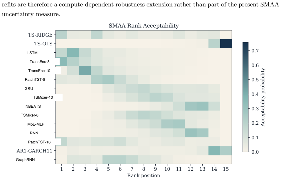
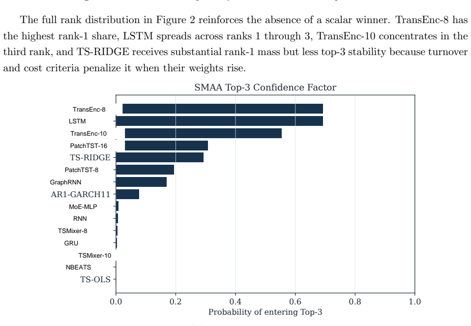
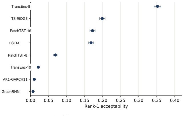
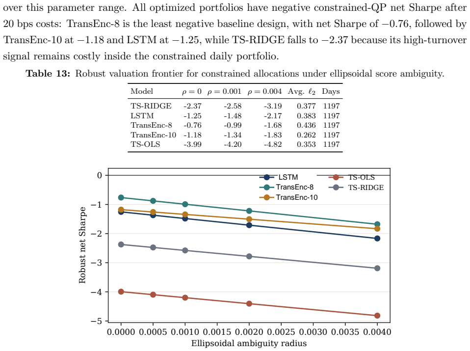
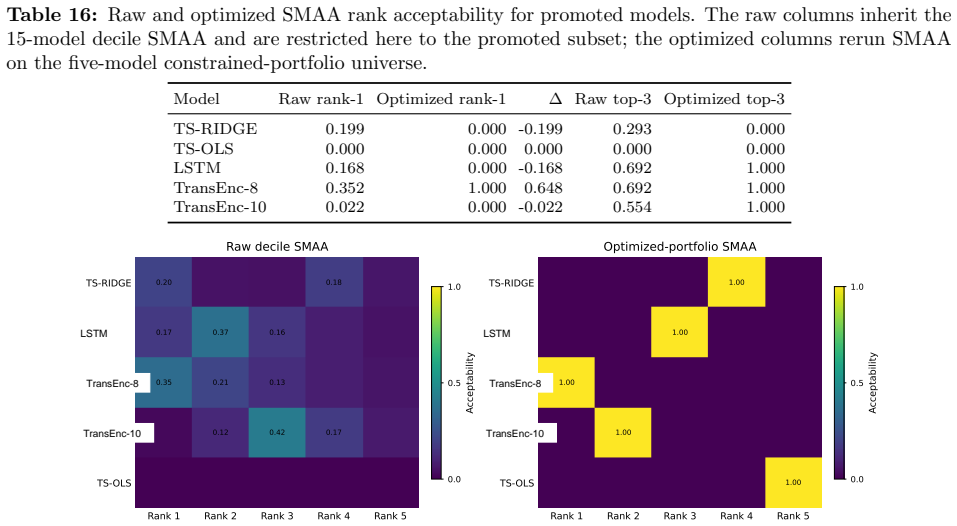
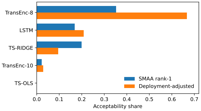
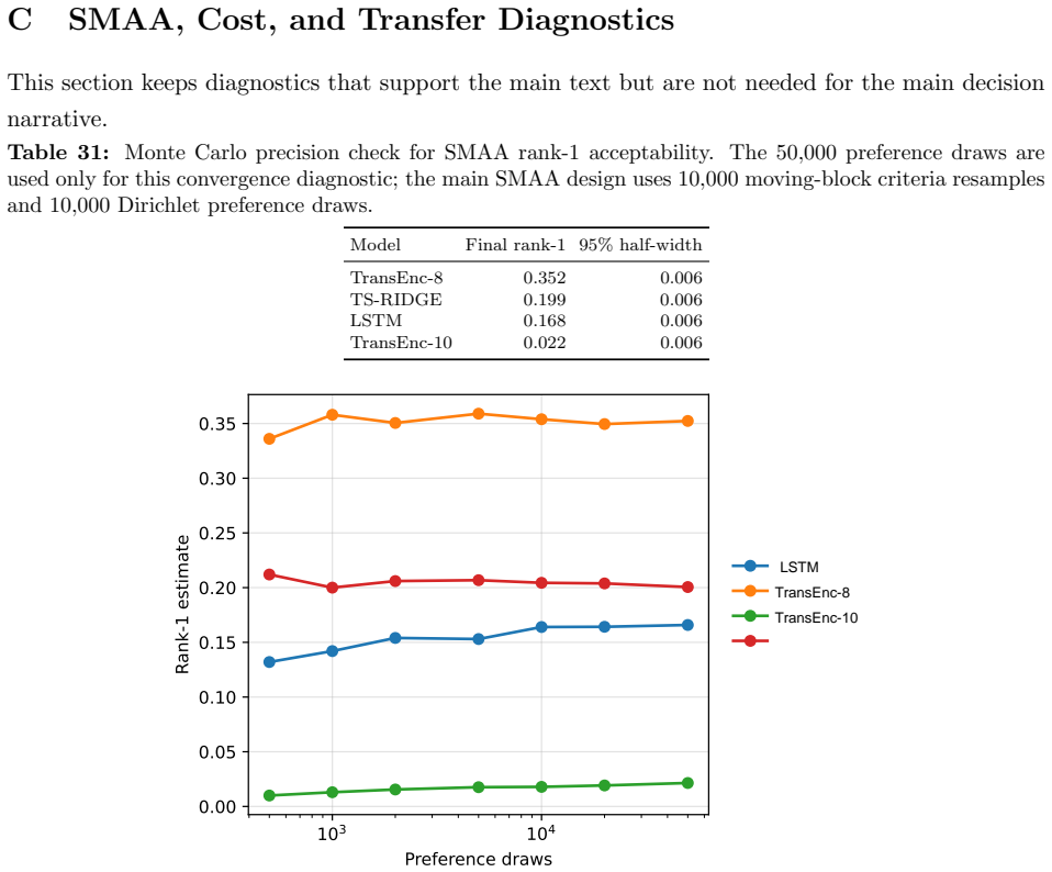
Benchmarking forecasting architectures for daily equity portfolios is not just a prediction exercise. It also asks which model remains usable after preferences, costs, and portfolio constraints are imposed. We build a CRSP daily-stock benchmark for 15 deep and statistical time-series architectures over 2018--2024. The protocol combines common-window decile portfolios, stochastic multi-criteria acceptability analysis, a deployment-adjusted acceptability index defined as an entropic update from the SMAA prior, and a constrained quadratic portfolio layer with capacity, beta, industry, risk, leverage, and turnover controls. Empirically, no architecture dominates the raw benchmark: TransEnc-8 has
What carries the argument
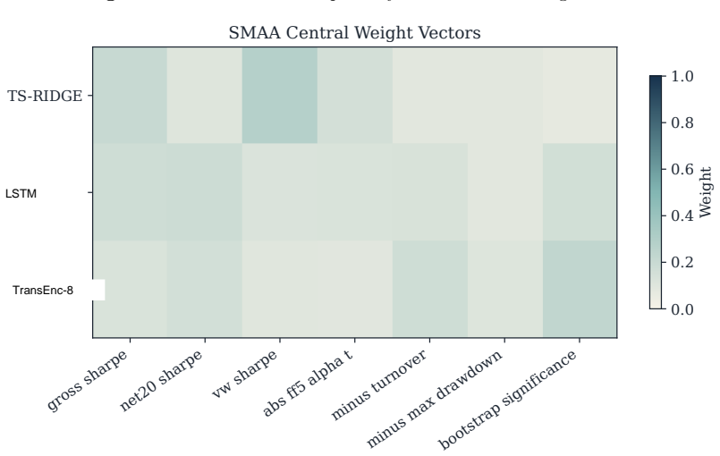
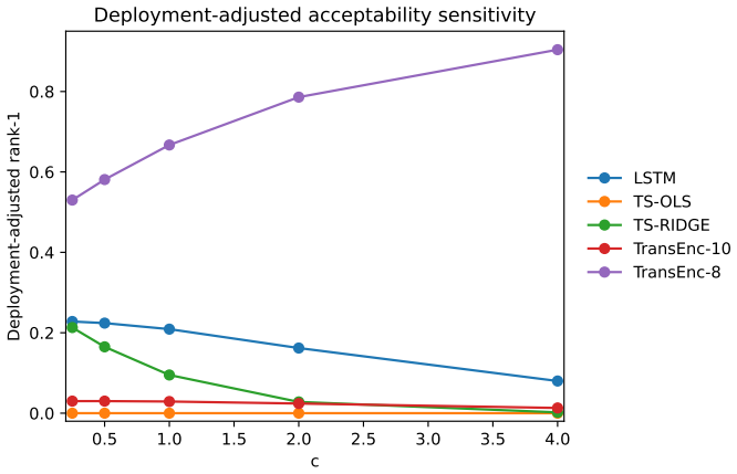
The deployment-adjusted acceptability index as an entropic update from the SMAA prior, applied to decile portfolios before constrained quadratic optimization with capacity, beta, industry, risk, leverage, and turnover controls.
If this is right
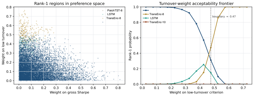
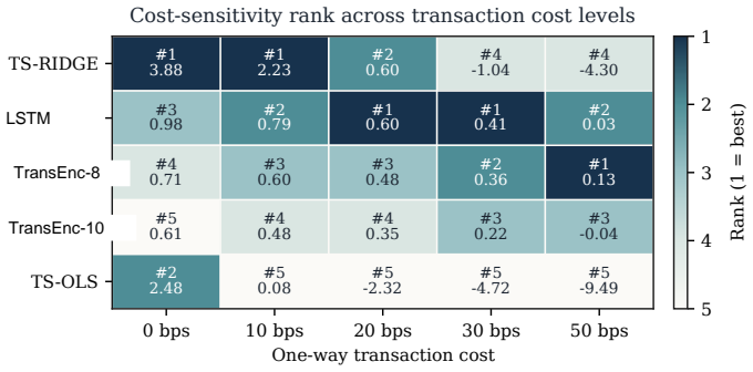
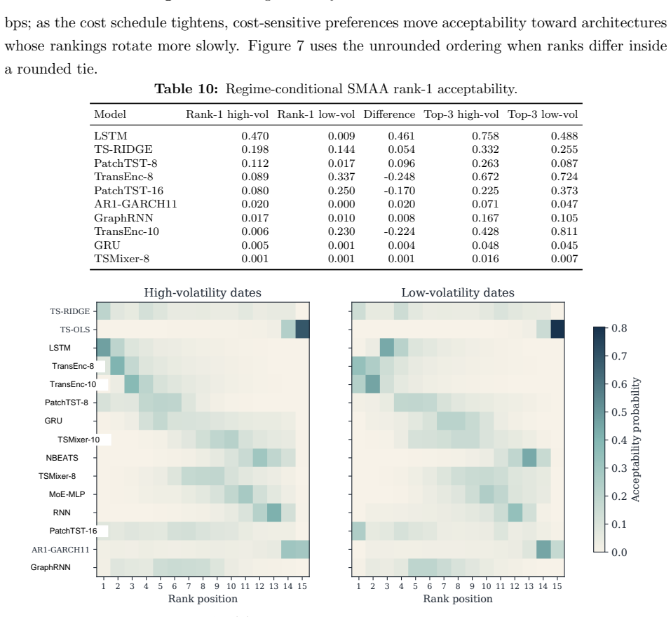
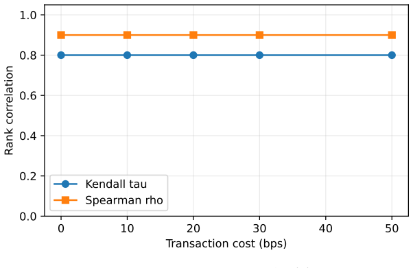
- Model rankings change with investor preferences, market state, feature universe, and transaction costs.
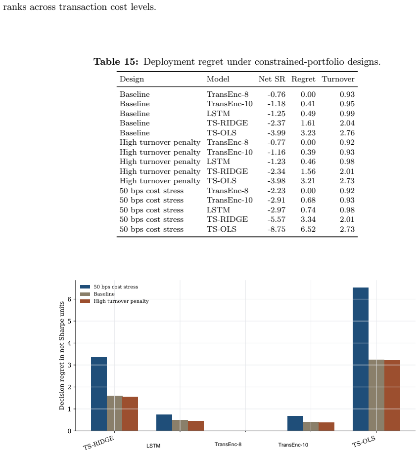
- TransEnc-8 is selected in the five-model constrained-portfolio comparison under the full protocol.
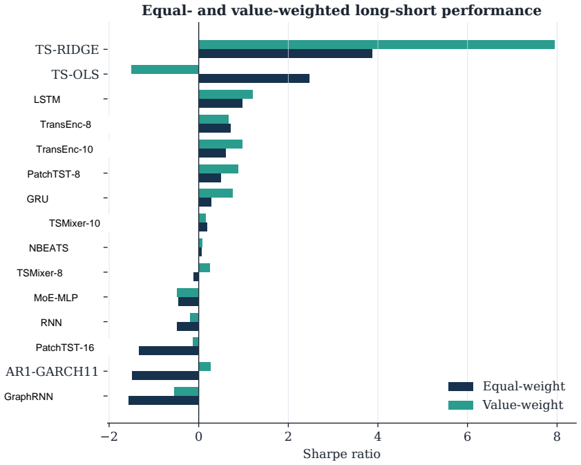
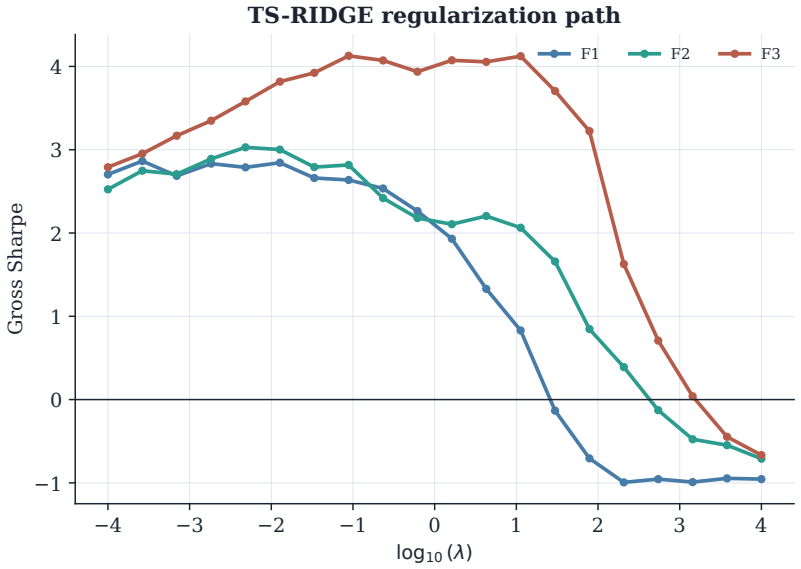
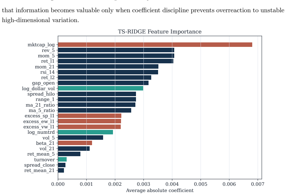
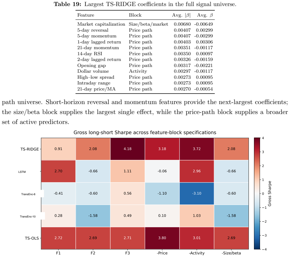
- Raw return-oriented rankings can instead favor TS-RIDGE.
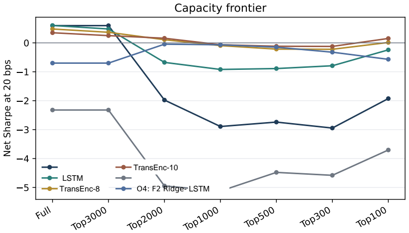
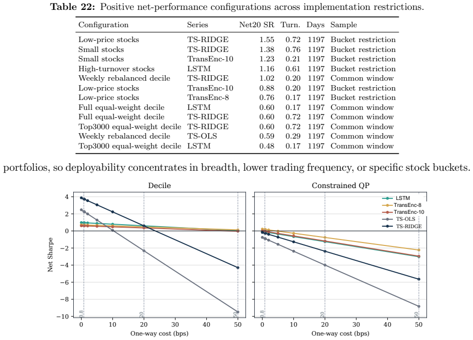
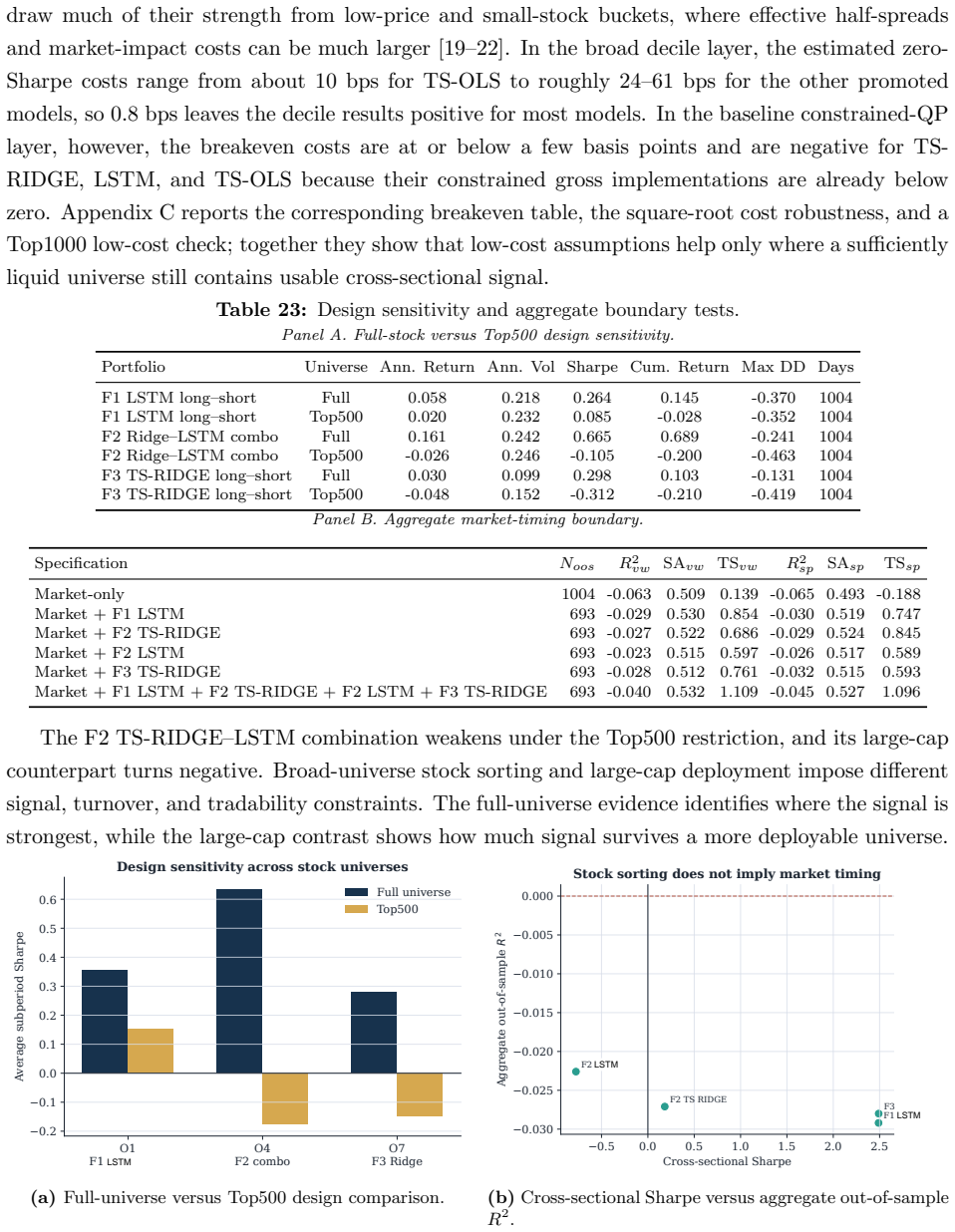
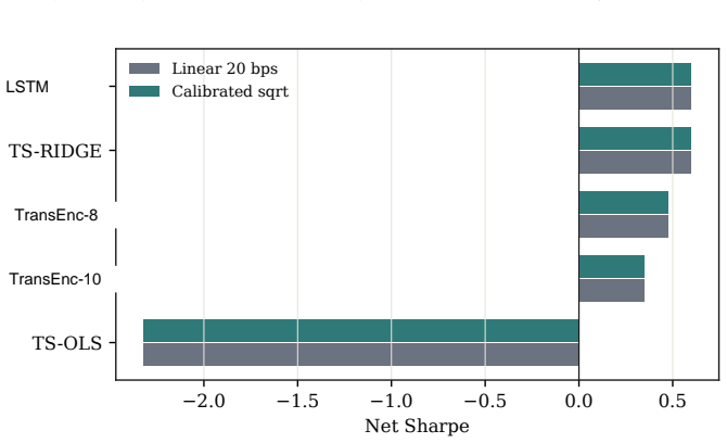
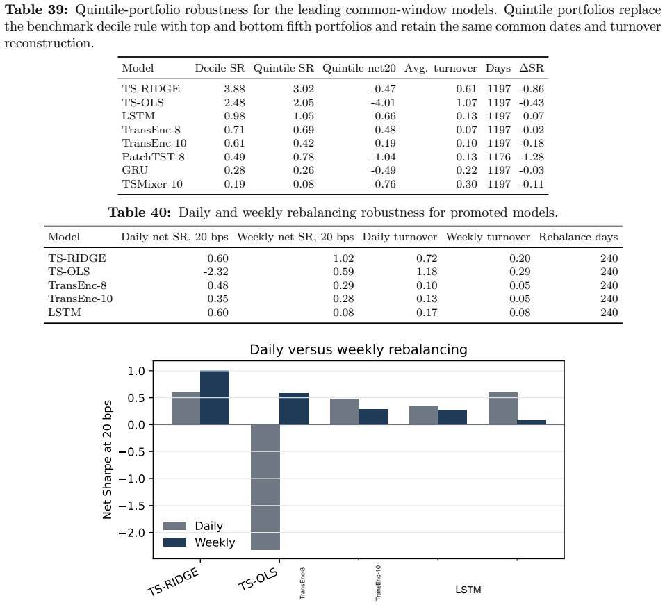
- Broad-universe decile signals survive costs in some configurations.
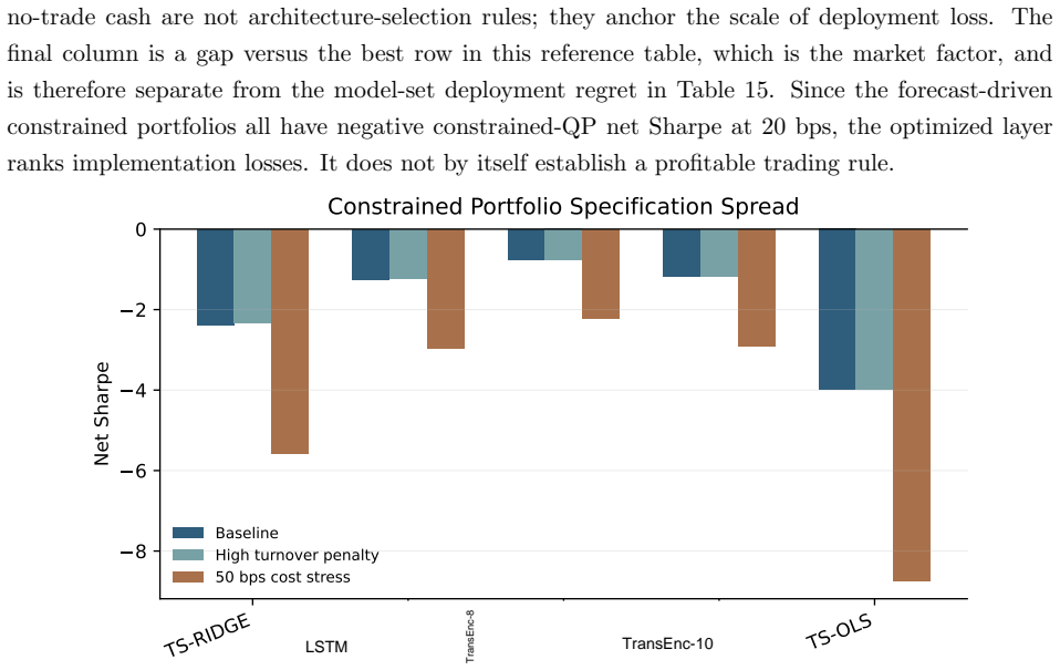
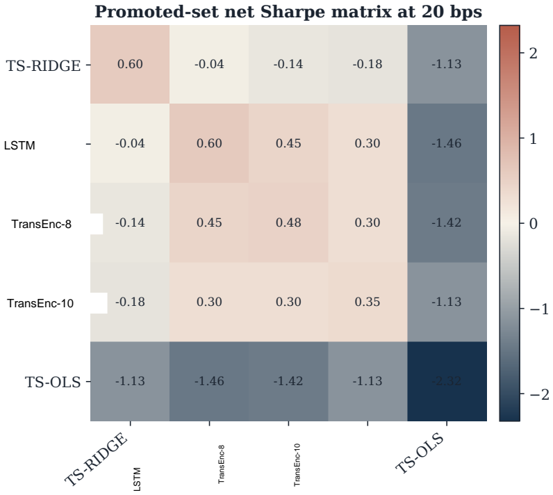
- Net Sharpe ratios after 20 bps costs are negative for all models in the baseline constrained QP.
Where Pith is reading between the lines
- Model selection for portfolios should incorporate full construction pipelines rather than isolated accuracy metrics.
- The entropic index could be tested on other multi-criteria problems such as credit or macro forecasting.
- Extending the protocol to intraday data or international equities would reveal whether the no-dominance result holds outside daily U.S. stocks.
Load-bearing premise
The protocol of common-window decile portfolios, SMAA, entropic acceptability index, and constrained QP with the listed controls is sufficient to determine which models remain usable after preferences, costs, and constraints are imposed.
What would settle it
Finding one architecture that produces positive net Sharpe ratios in the constrained QP across multiple preference weightings and cost levels would show dominance where the paper reports none.
Figures
read the original abstract
Benchmarking forecasting architectures for daily equity portfolios is not just a prediction exercise. It also asks which model remains usable after preferences, costs, and portfolio constraints are imposed. We build a CRSP daily-stock benchmark for 15 deep and statistical time-series architectures over 2018--2024. The protocol combines common-window decile portfolios, stochastic multi-criteria acceptability analysis, a deployment-adjusted acceptability index, and a constrained quadratic portfolio layer with capacity, beta, industry, risk, leverage, and turnover controls. The index starts from the SMAA rank-acceptability distribution and downweights models whose criteria-level wins produce high portfolio regret; its Gibbs form is characterized as an entropic update from the SMAA prior. Empirically, no architecture dominates the raw benchmark: TransEnc-8 has the largest rank-1 acceptability, 0.352, and no model exceeds about 0.36. Rankings vary with preferences, market state, feature universe, and transaction costs. In the promoted five-model constrained-portfolio comparison, TransEnc-8 is selected throughout, while return-oriented raw rankings can favor TS-RIDGE. Broad-universe decile signals can survive costs, but the baseline constrained-QP net Sharpe at 20 bps is negative for every promoted model. The benchmark supports model selection and diagnosis rather than a standalone trading-strategy claim.
Editorial analysis
A structured set of objections, weighed in public.
Referee Report
Summary. The paper benchmarks 15 deep and statistical time-series architectures for daily equity portfolio construction on CRSP data (2018–2024). It deploys a multi-stage protocol that constructs common-window decile portfolios, applies stochastic multi-criteria acceptability analysis (SMAA), defines a deployment-adjusted acceptability index via an entropic (Gibbs) update from the SMAA prior, and solves a constrained quadratic program incorporating capacity, beta, industry, risk, leverage, and turnover limits. The central empirical claims are that no architecture dominates (TransEnc-8 attains the highest rank-1 acceptability of 0.352; no model exceeds ~0.36), that rankings are sensitive to preferences, market state, feature universe, and transaction costs, that TransEnc-8 is selected in the five-model constrained comparison while return-oriented rankings can favor TS-RIDGE, and that broad-universe decile signals can survive costs yet the baseline constrained-QP net Sharpe at 20 bps remains negative for every promoted model.
Significance. If the protocol and implementation details hold, the work supplies a reproducible, preference-aware evaluation framework that moves beyond raw forecast accuracy to usability under realistic portfolio constraints. It credits the use of standard CRSP data, explicit multi-criteria SMAA, the explicit entropic characterization of the acceptability index, and the full set of QP controls. The negative net-Sharpe finding and the observation that no model dominates are falsifiable, policy-relevant results that caution against over-reliance on any single architecture.
minor comments (3)
- Abstract and §4: the exact functional form of the entropic update (Gibbs distribution) from the SMAA rank-acceptability vector to the deployment-adjusted index should be written explicitly, including the temperature parameter and any normalization, so that the index can be reproduced from the reported acceptability numbers alone.
- §3.3 and Table 2: the precise definition of the five-model constrained-QP comparison (which models are included, how the capacity and turnover limits are set, and whether the same random seeds are used across architectures) needs a dedicated paragraph or pseudocode block to eliminate ambiguity in the reported selection of TransEnc-8.
- Figure 3 and §5.2: the market-state and transaction-cost sensitivity plots would benefit from error bars or bootstrap intervals on the acceptability values so that the claim “rankings vary” can be assessed for statistical significance rather than visual inspection alone.
Simulated Author's Rebuttal
We thank the referee for the careful summary of the manuscript, the positive evaluation of its significance, and the recommendation of minor revision. No major comments appear in the report, so we provide no point-by-point rebuttals below. Any minor suggestions will be incorporated in the revised version.
Circularity Check
No significant circularity; empirical claims rest on external data and stated definitions
full rationale
The paper is an empirical benchmarking exercise on CRSP data using common-window decile portfolios, SMAA rank-acceptability, a defined entropic deployment-adjusted index (explicitly characterized as an update from the SMAA prior), and constrained QP optimization with explicit controls. No derivation reduces by construction to fitted parameters or self-citations; the index form is stated rather than derived from the target results, and all performance numbers (e.g., rank-1 acceptability 0.352) are computed from external market data and standard portfolio layers. The protocol is presented as a composite method whose outputs are falsifiable against the data rather than tautological.
Axiom & Free-Parameter Ledger
Reference graph
Works this paper leans on
-
[1]
Risto Lahdelma and Pekka Salminen. SMAA-2: Stochastic multicriteria acceptability analysis for group decision making.Operations Research, 49(3):444–454, 2001. doi: 10.1287/opre.49.3. 444.11220. URL https://doi.org/10.1287/opre.49.3.444.11220
-
[2]
Tommi Tervonen and Jos´ e Rui Figueira. A survey on stochastic multicriteria acceptability analysis methods.Journal of Multi-Criteria Decision Analysis, 15(1–2):1–14, 2008. doi: 10.1 002/mcda.407. URL https://doi.org/10.1002/mcda.407
-
[3]
Salvatore Greco, Matthias Ehrgott, and Jos´ e Rui Figueira, editors.Multiple Criteria Decision Analysis: State of the Art Surveys, volume 233 ofInternational Series in Operations Research & Management Science. Springer, 2 edition, 2016. doi: 10.1007/978-1-4939-3094-4. URL https://doi.org/10.1007/978-1-4939-3094-4
-
[4]
Panos Xidonas, George Mavrotas, Constantin Zopounidis, and John Psarras. IPSSIS: An inte- grated multicriteria decision support system for equity portfolio construction and selection.Eu- ropean Journal of Operational Research, 210(2):398–409, 2011. doi: 10.1016/j.ejor.2010.08.028. URL https://doi.org/10.1016/j.ejor.2010.08.028
-
[5]
Adam N. Elmachtoub and Paul Grigas. Smart “predict, then optimize”.Management Science, 68(1):9–26, 2022. doi: 10.1287/mnsc.2020.3922. URL https://doi.org/10.1287/mnsc.2020.3922
-
[6]
Cambridge Univer- sity Press, Cambridge, 2006
Nicolo Cesa-Bianchi and Gabor Lugosi.Prediction, Learning, and Games. Cambridge Univer- sity Press, Cambridge, 2006
2006
-
[7]
Robust portfolio selection problems.Mathematics of Operations Research, 28(1):1–38, 2003
Donald Goldfarb and Garud Iyengar. Robust portfolio selection problems.Mathematics of Operations Research, 28(1):1–38, 2003. doi: 10.1287/moor.28.1.1.14260. URL https://doi.org/ 10.1287/moor.28.1.1.14260
-
[8]
Erick Delage and Yinyu Ye. Distributionally robust optimization under moment uncertainty with application to data-driven problems.Operations Research, 58(3):595–612, 2010. doi: 10.1287/opre.1090.0741. URL https://doi.org/10.1287/opre.1090.0741
-
[9]
European Journal of Operational Research , author =
Dimitris Bertsimas and Martin S. Copenhaver. Characterization of the equivalence of ro- bustification and regularization in linear and matrix regression.European Journal of Op- erational Research, 270(3):931–942, 2018. doi: 10.1016/j.ejor.2017.03.051. URL https: //doi.org/10.1016/j.ejor.2017.03.051
-
[10]
Jose Blanchet, Yang Kang, and Karthyek Murthy. Robust wasserstein profile inference and applications to machine learning.Journal of Applied Probability, 56(3):830–857, 2019. doi: 10.1017/jpr.2019.49. URL https://doi.org/10.1017/jpr.2019.49. 47
-
[11]
Regularization via mass transportation.Journal of Machine Learning Research, 20(103):1–68, 2019
Soroosh Shafieezadeh-Abadeh, Daniel Kuhn, and Peyman Mohajerin Esfahani. Regularization via mass transportation.Journal of Machine Learning Research, 20(103):1–68, 2019. URL https://www.jmlr.org/papers/v20/17-633.html
2019
-
[12]
Giorgio Costa and Garud N. Iyengar. Distributionally robust end-to-end portfolio construction. Quantitative Finance, 23(10):1465–1482, 2023. doi: 10.1080/14697688.2023.2236148. URL https://doi.org/10.1080/14697688.2023.2236148
-
[13]
Fr´ ed´ eric Bonnans and Alexander Shapiro.Perturbation Analysis of Optimization Problems
J. Fr´ ed´ eric Bonnans and Alexander Shapiro.Perturbation Analysis of Optimization Problems. Springer, 2000. doi: 10.1007/978-1-4612-1394-9. URL https://doi.org/10.1007/978-1-4612-1 394-9
-
[14]
Elmachtoub, Paul Grigas, and Ambuj Tewari
Othman El Balghiti, Adam N. Elmachtoub, Paul Grigas, and Ambuj Tewari. Generalization bounds in the predict-then-optimize framework. InAdvances in Neural Information Processing Systems, volume 32, 2019. URL https://proceedings.neurips.cc/paper/2019/hash/a70145bf8b1 73e4496b554ce57969e24-Abstract.html
2019
-
[15]
Topkis.Supermodularity and Complementarity
Donald M. Topkis.Supermodularity and Complementarity. Princeton University Press, 1998. URL https://press.princeton.edu/books/paperback/9780691032443/supermodularity-and-com plementarity
arXiv 1998
-
[16]
Shihao Gu, Bryan Kelly, and Dacheng Xiu. Empirical asset pricing via machine learning. The Review of Financial Studies, 33(5):2223–2273, 2020. doi: 10.1093/rfs/hhaa009. URL https://doi.org/10.1093/rfs/hhaa009
-
[17]
Deep learning in asset pricing.Management Science, 70(2):714–750, 2024
Luyang Chen, Markus Pelger, and Jason Zhu. Deep learning in asset pricing.Management Science, 70(2):714–750, 2024. doi: 10.1287/mnsc.2023.4695. URL https://doi.org/10.1287/mn sc.2023.4695
-
[18]
Doron Avramov, Si Cheng, and Lior Metzker. Machine learning versus economic restrictions: Evidence from stock return predictability.Management Science, 69(5):2587–2619, 2023. doi: 10.1287/mnsc.2022.4449. URL https://doi.org/10.1287/mnsc.2022.4449
-
[19]
Victor DeMiguel, Alberto Mart´ ın-Utrera, Francisco J. Nogales, and Raman Uppal. A transaction-cost perspective on the multitude of firm characteristics.The Review of Finan- cial Studies, 33(5):2180–2222, 2020. doi: 10.1093/rfs/hhz085. URL https://doi.org/10.1093/rf s/hhz085
-
[20]
Model comparison with transaction costs.The Journal of Finance, 78(3):1743–1775, 2023
Andrew Detzel, Robert Novy-Marx, and Mihail Velikov. Model comparison with transaction costs.The Journal of Finance, 78(3):1743–1775, 2023. doi: 10.1111/jofi.13225. URL https: //doi.org/10.1111/jofi.13225
-
[21]
Andrew Y. Chen and Mihail Velikov. Zeroing in on the expected returns of anomalies.Journal of Financial and Quantitative Analysis, 58(3):968–1004, 2023. doi: 10.1017/S0022109022000874. URL https://doi.org/10.1017/S0022109022000874
-
[22]
Andrea Frazzini, Ronen Israel, and Tobias J. Moskowitz. Trading costs.SSRN Electronic Journal, 2018. doi: 10.2139/ssrn.3229719. URL https://doi.org/10.2139/ssrn.3229719. 48
-
[23]
Asness, Andrea Frazzini, Ronen Israel, Tobias J
Clifford S. Asness, Andrea Frazzini, Ronen Israel, Tobias J. Moskowitz, and Lasse H. Pedersen. Size matters, if you control your junk.Journal of Financial Economics, 129(3):479–509, 2018. doi: 10.1016/j.jfineco.2018.05.006. URL https://doi.org/10.1016/j.jfineco.2018.05.006
-
[24]
Eugene F. Fama and Kenneth R. French. Common risk factors in the returns on stocks and bonds.Journal of Financial Economics, 33(1):3–56, 1993. doi: 10.1016/0304-405X(93)90023-5. URL https://doi.org/10.1016/0304-405X(93)90023-5
-
[25]
Eugene F. Fama and Kenneth R. French. A five-factor asset pricing model.Journal of Financial Economics, 116(1):1–22, 2015. doi: 10.1016/j.jfineco.2014.10.010. URL https://doi.org/10.101 6/j.jfineco.2014.10.010
-
[26]
Digesting anomalies: An investment approach.The Review of Financial Studies, 28(3):650–705, 2015
Kewei Hou, Chen Xue, and Lu Zhang. Digesting anomalies: An investment approach.The Review of Financial Studies, 28(3):650–705, 2015. doi: 10.1093/rfs/hhu068. URL https: //doi.org/10.1093/rfs/hhu068
-
[27]
An augmented q-factor model with expected growth.Review of Finance, 25(1):1–41, 2021
Kewei Hou, Haitao Mo, Chen Xue, and Lu Zhang. An augmented q-factor model with expected growth.Review of Finance, 25(1):1–41, 2021. doi: 10.1093/rof/rfaa004. URL https://doi.org/ 10.1093/rof/rfaa004
-
[28]
Robert Novy-Marx. The other side of value: The gross profitability premium.Journal of Financial Economics, 108(1):1–28, 2013. doi: 10.1016/j.jfineco.2013.01.003. URL https: //doi.org/10.1016/j.jfineco.2013.01.003
-
[29]
David McLean and Jeffrey Pontiff
R. David McLean and Jeffrey Pontiff. Does academic research destroy stock return pre- dictability?The Journal of Finance, 71(1):5–32, 2016. doi: 10.1111/jofi.12365. URL https://doi.org/10.1111/jofi.12365
-
[30]
Replicating anomalies.The Review of Financial Studies, 33(5):2019–2133, 2020
Kewei Hou, Chen Xue, and Lu Zhang. Replicating anomalies.The Review of Financial Studies, 33(5):2019–2133, 2020. doi: 10.1093/rfs/hhy131. URL https://doi.org/10.1093/rfs/hhy131
-
[31]
Andrew Y. Chen and Tom Zimmermann. Open source cross-sectional asset pricing.Critical Finance Review, 11(2):207–264, 2022. doi: 10.1561/104.00000112. URL https://doi.org/10.156 1/104.00000112
-
[32]
Webb, Rob J
Rakshitha Godahewa, Christoph Bergmeir, Geoffrey I. Webb, Rob J. Hyndman, and Pablo Montero-Manso. Monash time series forecasting archive. InProceedings of the Neural Informa- tion Processing Systems Track on Datasets and Benchmarks, 2021. URL https://openreview.n et/forum?id=I01l7rc0jcb
2021
-
[33]
M5 accuracy competi- tion: Results, findings, and conclusions.International Journal of Forecasting, 38(4):1346–1364,
Spyros Makridakis, Evangelos Spiliotis, and Vassilios Assimakopoulos. M5 accuracy competi- tion: Results, findings, and conclusions.International Journal of Forecasting, 38(4):1346–1364,
-
[34]
doi: 10.1016/j.ijforecast.2021.11.013. URL https://doi.org/10.1016/j.ijforecast.2021.11.0 13
-
[35]
Arik, Nicolas Loeff, and Tomas Pfister
Bryan Lim, Sercan ¨O. Arik, Nicolas Loeff, and Tomas Pfister. Temporal fusion transformers for interpretable multi-horizon time series forecasting.International Journal of Forecasting, 37 (4):1748–1764, 2021. doi: 10.1016/j.ijforecast.2021.03.012. URL https://doi.org/10.1016/j.ijfo recast.2021.03.012. 49
-
[36]
Oreshkin, Dmitri Carpov, Nicolas Chapados, and Yoshua Bengio
Boris N. Oreshkin, Dmitri Carpov, Nicolas Chapados, and Yoshua Bengio. N-BEATS: Neural basis expansion analysis for interpretable time series forecasting. InInternational Conference on Learning Representations, 2020. URL https://openreview.net/forum?id=r1ecqn4YwB. Published as a conference paper at ICLR 2020; arXiv:1905.10437
arXiv 2020
-
[37]
Ailing Zeng, Muxi Chen, Lei Zhang, and Qiang Xu. Are transformers effective for time series forecasting? InProceedings of the AAAI Conference on Artificial Intelligence, volume 37, pages 11121–11128, 2023. doi: 10.1609/aaai.v37i9.26317. URL https://doi.org/10.1609/aaai.v37i9.2 6317
-
[38]
Kashif Rasul, Arjun Ashok, Andrew Robert Williams, Hena Ghonia, Rishika Bhagwatkar, Arian Khorasani, Mohammad Javad Darvishi Bayazi, George Adamopoulos, Roland Riachi, Nadhir Hassen, Marin Biloˇ s, Sahil Garg, Anderson Schneider, Nicolas Chapados, Alexandre Drouin, Valentina Zantedeschi, Yuriy Nevmyvaka, and Irina Rish. Lag-Llama: Towards foundation model...
-
[39]
Gift-eval: A benchmark for general time series forecasting model evaluation
Taha Aksu, Gerald Woo, Juncheng Liu, Xu Liu, Chenghao Liu, Silvio Savarese, Caiming Xiong, and Doyen Sahoo. Gift-eval: A benchmark for general time series forecasting model evaluation. arXiv preprint arXiv:2410.10393, 2024. doi: 10.48550/arXiv.2410.10393. URL https://arxiv. org/abs/2410.10393
-
[40]
Andrew W. Lo. The statistics of sharpe ratios.Financial Analysts Journal, 58(4):36–52, 2002. doi: 10.2469/faj.v58.n4.2453. URL https://doi.org/10.2469/faj.v58.n4.2453
-
[41]
Robust performance hypothesis testing with the sharpe ratio
Olivier Ledoit and Michael Wolf. Robust performance hypothesis testing with the sharpe ratio. Journal of Empirical Finance, 15(5):850–859, 2008. doi: 10.1016/j.jempfin.2008.03.002. URL https://doi.org/10.1016/j.jempfin.2008.03.002
-
[42]
Whitney K. Newey and Kenneth D. West. A simple, positive semi-definite, heteroskedasticity and autocorrelation consistent covariance matrix.Econometrica, 55(3):703–708, 1987. URL https://www.jstor.org/stable/1913610
arXiv 1987
-
[43]
of” in the title, which we felt was better than the original, “on
Halbert White. A reality check for data snooping.Econometrica, 68(5):1097–1126, 2000. doi: 10.1111/1468-0262.00152. URL https://doi.org/10.1111/1468-0262.00152
-
[44]
Peter R. Hansen. A test for superior predictive ability.Journal of Business & Economic Statistics, 23(4):365–380, 2005. doi: 10.1198/073500105000000063. URL https://doi.org/10.1 198/073500105000000063
-
[45]
Joseph P. Romano and Michael Wolf. Stepwise multiple testing as formalized data snooping. Econometrica, 73(4):1237–1282, 2005. doi: 10.1111/j.1468-0262.2005.00615.x. URL https: //doi.org/10.1111/j.1468-0262.2005.00615.x
-
[46]
and Lunde, Asger and Nason, James M
Peter R. Hansen, Asger Lunde, and James M. Nason. The model confidence set.Econometrica, 79(2):453–497, 2011. doi: 10.3982/ECTA5771. URL https://doi.org/10.3982/ECTA5771
-
[47]
Francis X. Diebold and Roberto S. Mariano. Comparing predictive accuracy.Journal of Busi- ness & Economic Statistics, 13(3):253–263, 1995. doi: 10.1080/07350015.1995.10524599. URL https://doi.org/10.1080/07350015.1995.10524599. 50
-
[48]
Harvey, Yan Liu, and Heqing Zhu
Campbell R. Harvey, Yan Liu, and Heqing Zhu. ... and the cross-section of expected returns. The Review of Financial Studies, 29(1):5–68, 2016. doi: 10.1093/rfs/hhv059. URL https: //doi.org/10.1093/rfs/hhv059
-
[49]
Peyman Mohajerin Esfahani and Daniel Kuhn. Data-driven distributionally robust optimization using the wasserstein metric: Performance guarantees and tractable reformulations.Math- ematical Programming, 171(1–2):115–166, 2018. doi: 10.1007/s10107-017-1172-1. URL https://doi.org/10.1007/s10107-017-1172-1
-
[50]
Dimitris N. Politis and Halbert White. Automatic block-length selection for the dependent bootstrap.Econometric Reviews, 23(1):53–70, 2004. doi: 10.1081/ETC-120028836. URL https://doi.org/10.1081/ETC-120028836
-
[51]
Shrinking the cross-section.Journal of Financial Economics, 135(2):271–292, 2020
Serhiy Kozak, Stefan Nagel, and Shrihari Santosh. Shrinking the cross-section.Journal of Financial Economics, 135(2):271–292, 2020. doi: 10.1016/j.jfineco.2019.06.008. URL https: //doi.org/10.1016/j.jfineco.2019.06.008. 51
discussion (0)
Sign in with ORCID, Apple, or X to comment. Anyone can read and Pith papers without signing in.