Explicit Quantum Circuit Simulation of Nonlinear 1-Dimensional Fluid with Carleman-linearized Boltzmann Method
Pith reviewed 2026-06-27 07:00 UTC · model grok-4.3
The pith
Second-order Carleman linearization of the one-dimensional Boltzmann equation lets quantum circuits prepare the final-time state of a nonlinear fluid via a QSVT-based Taylor ODE solver.
A machine-rendered reading of the paper's core claim, the machinery that carries it, and where it could break.
Core claim
By applying second-order Carleman linearization to the one-dimensional Boltzmann equation, the nonlinear fluid problem is turned into a linear system whose time evolution is solved by a Taylor-expansion-based ODE solver realized with quantum singular value transformation; explicit gate-level circuit simulation then prepares the final-time state, and the resulting gate and qubit complexities are shown to scale logarithmically with grid size, with the order of the Carleman truncation controlling the captured nonlinearity.
What carries the argument
second-order Carleman linearization of the one-dimensional Boltzmann equation together with a Taylor-expansion ODE solver implemented via quantum singular value transformation
If this is right
- Gate and qubit counts scale logarithmically with grid size.
- Higher-order Carleman expansions capture additional nonlinearity at the cost of larger but still logarithmic resources.
- The same construction supplies a baseline for reducing computational cost in future work.
- Extensions to higher dimensions, complex geometries, and extraction of physical quantities become concrete next targets once the one-dimensional nonlinear case is established.
Where Pith is reading between the lines
- The logarithmic scaling suggests that, if the truncation error remains controlled, the method could remain practical even when the spatial grid is refined to resolve finer flow features.
- Because the circuit is built from explicit elementary gates, one could in principle substitute a different linear-system solver or a different time integrator and measure the change in total gate count directly.
- If the second-order truncation proves accurate enough for selected benchmark flows, the same linearization step might be reusable as a modular component inside larger quantum CFD pipelines that add forcing terms or boundary conditions.
Load-bearing premise
The second-order truncation of the Carleman expansion produces a sufficiently accurate linear system whose solution on the quantum circuit corresponds to the true nonlinear fluid dynamics at the chosen grid resolution and time step.
What would settle it
Compare the final-time probability distribution or moments obtained from the explicit quantum circuit simulation against the output of a classical nonlinear lattice Boltzmann solver run at identical grid size, time step, and truncation order; systematic deviation beyond statistical error would falsify the claim that the quantum procedure reproduces the target nonlinear dynamics.
Figures
read the original abstract
Quantum computation of fluid dynamics has attracted growing attention as a key application of fault-tolerant quantum computers anticipated in the coming decade, with lattice Boltzmann methods emerging as a particularly promising approach. Explicit and efficient elementary-gate-level circuit simulations, however, have so far been demonstrated only in the linear case. Here we include the leading nonlinearity through second-order Carleman linearization of the one-dimensional Boltzmann equation, and demonstrate, via explicit quantum-circuit simulation, the preparation of the final-time state using a Taylor-expansion-based ODE solver based on the quantum singular value transformation. With this construction, we analyze the gate and qubit complexities, which scale logarithmically with the grid size, the nonlinearity captured by the higher-order Carleman linearization, and the practical utility of higher-order expansions in the Taylor ODE solver. The construction provides a concrete baseline for computational cost reduction and further developments such as extensions to higher dimensions, complex geometries, and the extraction of physical quantities, towards industrially useful quantum CFD.
Editorial analysis
A structured set of objections, weighed in public.
Referee Report
Summary. The manuscript constructs an explicit quantum circuit for simulating nonlinear one-dimensional fluid dynamics by applying second-order Carleman linearization to the Boltzmann equation and implementing a Taylor-expansion-based ODE solver via quantum singular value transformation (QSVD). It demonstrates preparation of the final-time state through explicit circuit simulation and analyzes the resulting gate and qubit complexities, which are claimed to scale logarithmically with grid size and the order of the Carleman expansion.
Significance. If the second-order Carleman truncation is shown to be sufficiently accurate, the work supplies a concrete, explicitly simulated baseline for quantum-circuit costs in nonlinear CFD with logarithmic scaling, which could inform extensions to higher dimensions and extraction of physical observables. The explicit simulation and complexity analysis are positive features.
major comments (2)
- [Abstract] Abstract: the central claim that the quantum circuit prepares a state corresponding to the nonlinear fluid dynamics rests on the second-order Carleman truncation producing a sufficiently accurate linear system, yet no a-priori error bound on the Carleman remainder is supplied and no direct numerical comparison against an independent classical integrator of the original nonlinear equation is reported.
- [Abstract] Abstract: the manuscript states the construction and scaling but supplies no numerical verification, error analysis, or comparison against a classical nonlinear solver, so the practical fidelity of the simulated state to the true nonlinear dynamics cannot be assessed from the provided material.
Simulated Author's Rebuttal
We thank the referee for their careful reading and constructive comments on the manuscript. We address the major comments point by point below.
read point-by-point responses
-
Referee: [Abstract] Abstract: the central claim that the quantum circuit prepares a state corresponding to the nonlinear fluid dynamics rests on the second-order Carleman truncation producing a sufficiently accurate linear system, yet no a-priori error bound on the Carleman remainder is supplied and no direct numerical comparison against an independent classical integrator of the original nonlinear equation is reported.
Authors: We agree that the manuscript does not supply an a-priori analytic bound on the Carleman remainder or a direct numerical comparison to a classical nonlinear integrator. The work centers on the explicit quantum-circuit construction and logarithmic complexity scaling for the second-order Carleman-linearized system; validation of truncation accuracy was outside the stated scope. In revision we will add a dedicated numerical section that compares the second-order Carleman solution against an independent classical nonlinear Boltzmann solver on the same 1-D test problems, together with a discussion of observed truncation error. revision: yes
-
Referee: [Abstract] Abstract: the manuscript states the construction and scaling but supplies no numerical verification, error analysis, or comparison against a classical nonlinear solver, so the practical fidelity of the simulated state to the true nonlinear dynamics cannot be assessed from the provided material.
Authors: This observation is correct. The explicit circuit simulation and scaling analysis are performed on the Carleman-linearized ODE; no direct fidelity check against the original nonlinear dynamics is reported. We will revise the manuscript to include such numerical verification and error assessment so that readers can evaluate the practical accuracy of the second-order truncation for the chosen test cases. revision: yes
Circularity Check
No significant circularity in derivation chain
full rationale
The paper constructs an explicit quantum circuit for the Carleman-linearized 1D Boltzmann equation via a Taylor-expansion ODE solver based on QSVD. All steps are presented as direct applications of established primitives (Carleman truncation, QSVD, Taylor series) without any reduction of the central claim to a fitted parameter, self-citation load-bearing premise, or input-by-construction. The derivation remains self-contained; external validation of truncation accuracy is a separate correctness issue, not a circularity defect.
Axiom & Free-Parameter Ledger
axioms (1)
- domain assumption Second-order Carleman linearization sufficiently approximates the nonlinear Boltzmann collision term for the 1D fluid problem
Reference graph
Works this paper leans on
-
[1]
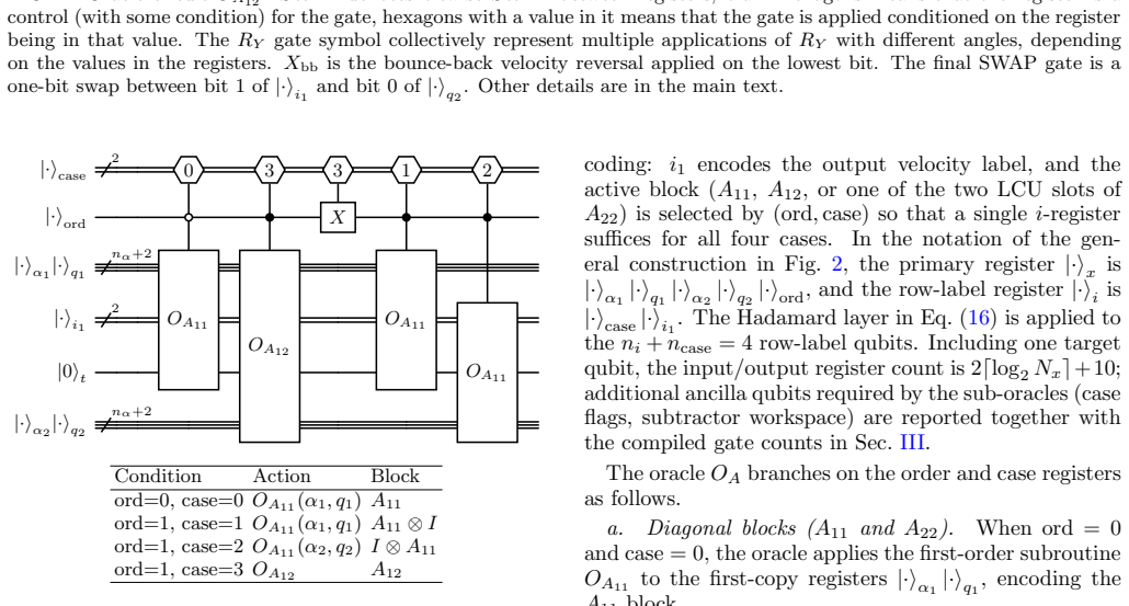
Figure 4 shows the circuit structure of theA 12 oracle, and Fig
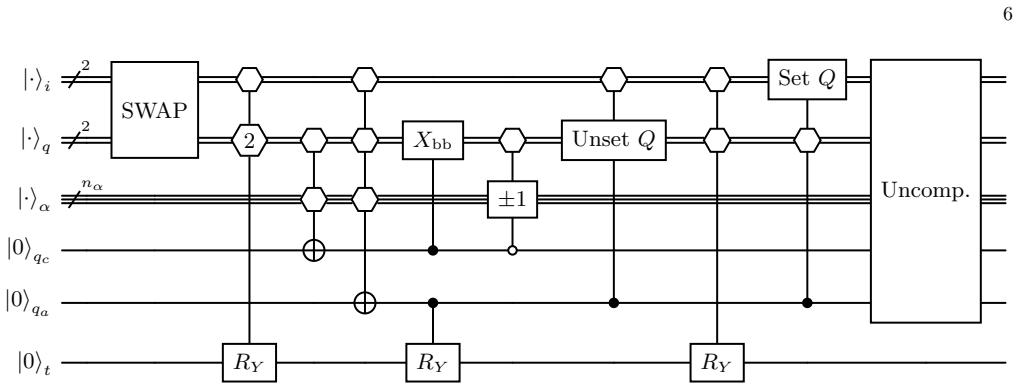
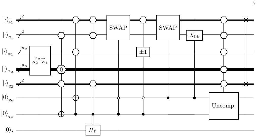
Second-order block encoding (U A forN C = 2) At second-order Carleman truncation, the block en- coding must implement the full rate matrix (11) with three nontrivial blocks: the diagonal blocksA 11 and A22 =A 11 ⊗I+I⊗A 11, and the off-diagonal block A12 encoding the nonlinear collision coupling fromf (2) tof (1). Figure 4 shows the circuit structure of th...
-
[2]
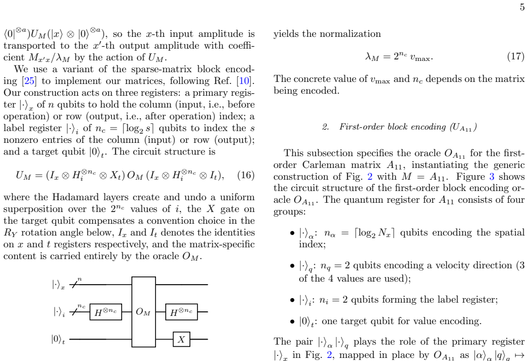
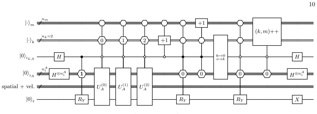
1) is implemented using theA-matrix oracles of Sec
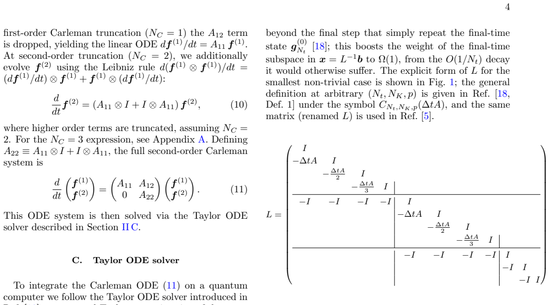
Block encoding ofL The block encodingU L of the time-evolution matrix L(Fig. 1) is implemented using theA-matrix oracles of Sec. II D 2 and II D 3 as controlled subroutines. The block encoding ofLrequires a Taylor-index regis- ter|·⟩ k ofn k =⌈log 2(NK+1)⌉qubits, a time-step register |·⟩m ofn m =⌈log 2(Nt)+1⌉qubits, and a composite row- label register who...
-
[3]
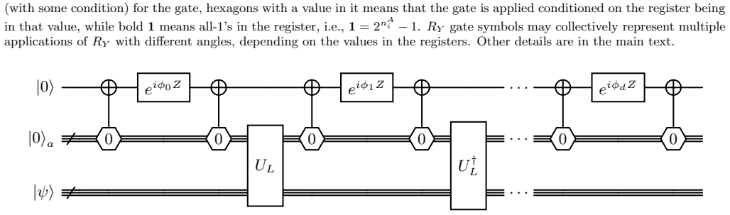
QSVT applies a polynomial transformationp(σ) to each sin- gular valueσof the block-encoded matrix
SolvingLx=bvia QSVT The linear systemLx=bis solved using the quan- tum singular value transformation (QSVT) [19]. QSVT applies a polynomial transformationp(σ) to each sin- gular valueσof the block-encoded matrix. By choos- ingp(σ)≈1/σ(a polynomial approximation to the in- verse function), we implementL −1 as a quantum cir- cuit. The QSVT circuit alternate...
-
[4]
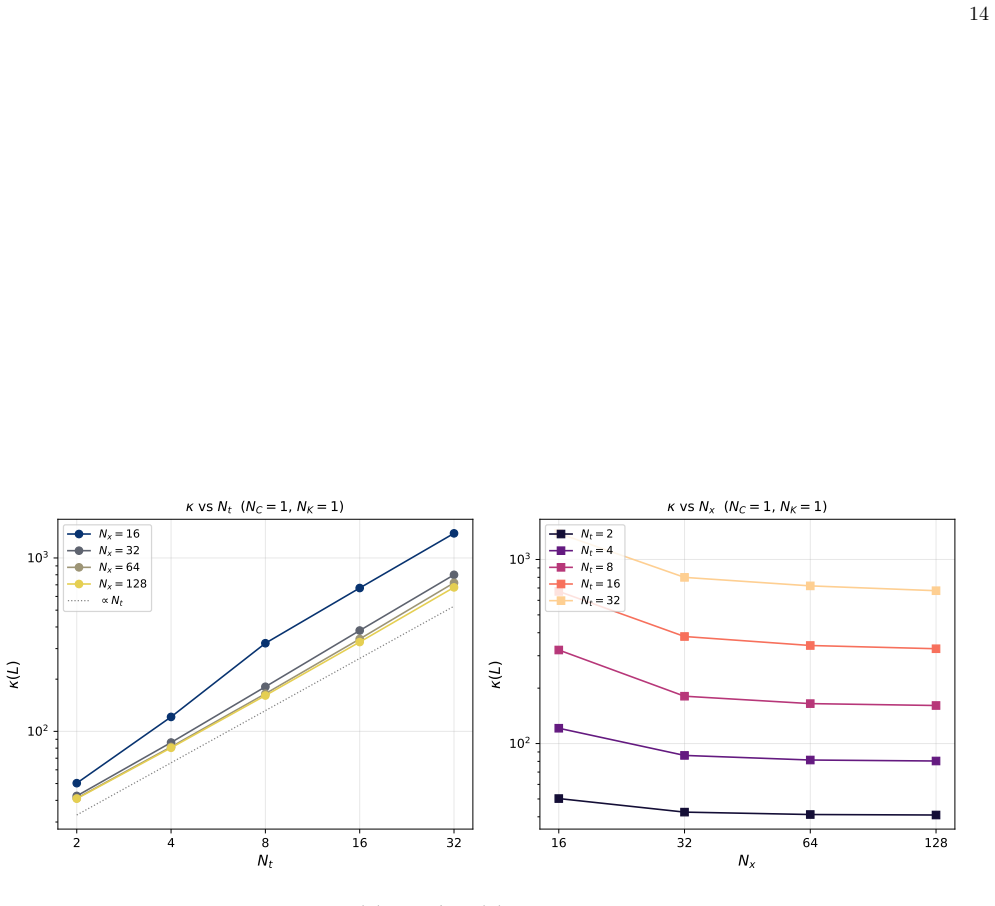
At fixedN t (right panel),κ(L) de- cays with increasingN x to a constant value
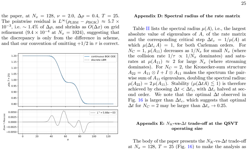
Dependence onN x andN t Figure 13 showsκ(L) atN C = 1,N K = 1 as a func- tion ofN t andN x. At fixedN t (right panel),κ(L) de- cays with increasingN x to a constant value. This satu- ration reflects theN x dependence of the spectral radius µ(A) of the rate matrix (Appendix D):µ(A)∝1/N x when the collision rate 1/τdominates (smallN x, via Eq. (18)), andµ(A...
-
[5]
Half 5 of this comes from 5 The rest is attributed to the decrease in the smallest singular value
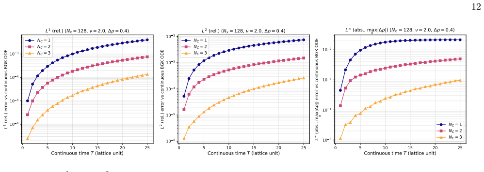
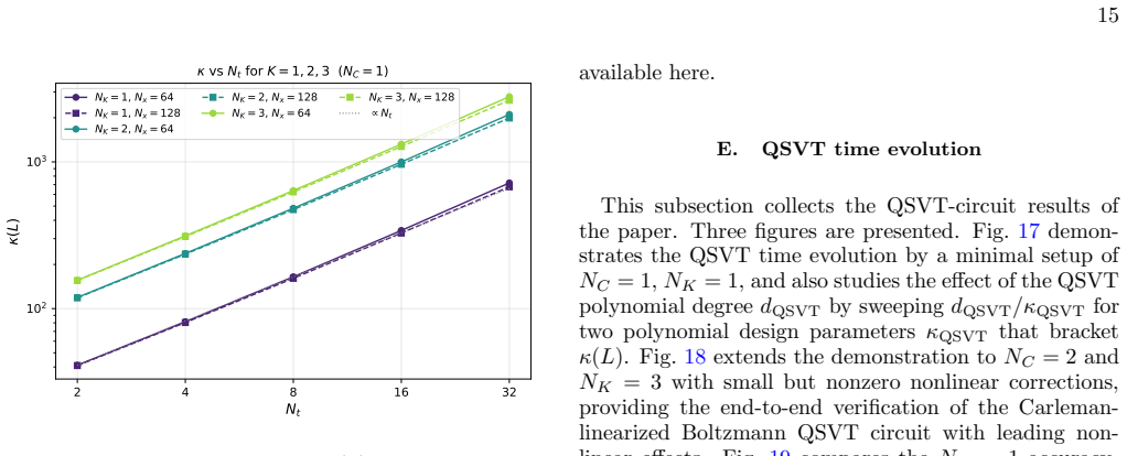
Dependence on the Taylor truncation orderN K Figure 14 showsκ(L) forN K = 1,2,3 acrossN x ∈ {64,128}andN t ∈ {2,4,8,16}: the linearκ(L)∝N t scaling persists for eachN K, andκ NK=3/κNK=1 ∼4 throughout the stable regime. Half 5 of this comes from 5 The rest is attributed to the decrease in the smallest singular value. 12 0 5 10 15 20 25 Continuous time T (l...
-
[6]
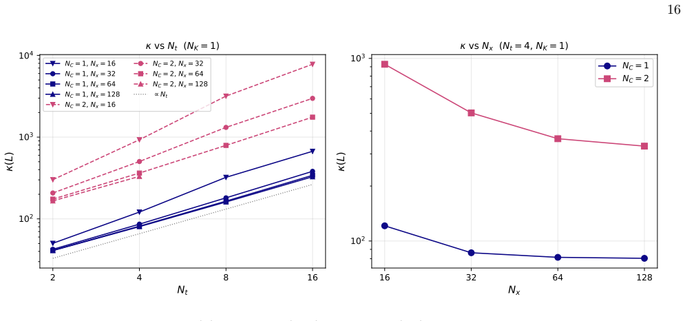
The spectral radiusµ(A) is exactly 2×itsN C = 1 value, which shifts the stable regime to largerN x
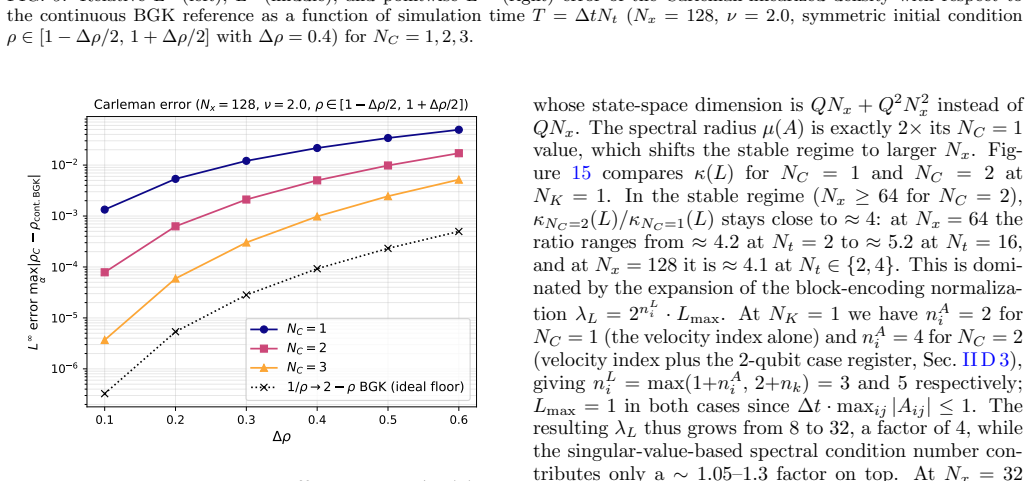
Dependence on the Carleman orderN C Extending the analysis to the second-order Carleman (NC = 2) requires solving an enlarged linear system whose state-space dimension isQN x +Q 2N2 x instead of QNx. The spectral radiusµ(A) is exactly 2×itsN C = 1 value, which shifts the stable regime to largerN x. Fig- ure 15 comparesκ(L) forN C = 1 andN C = 2 at NK = 1....
-
[7]
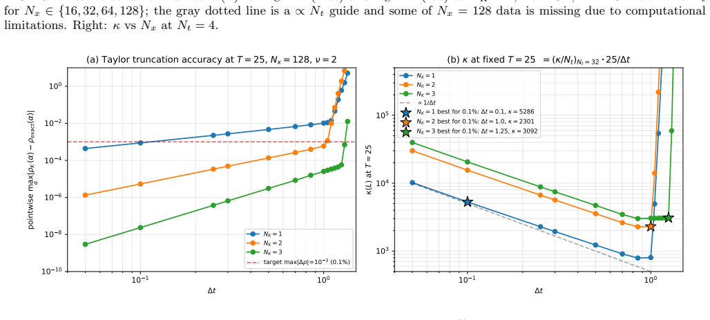
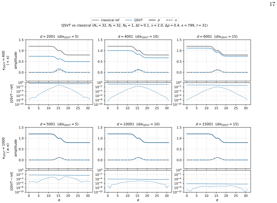
QSVT simulation with variousd QSVT andκ QSVT We perform a state-vector simulation of the full QSVT circuit atN x = 32,N t = 32 (first-order CarlemanN C = 1,N K = 1, ∆t= 0.1), using theL-matrix QSVT circuit of Sec. II D 5. The effective condition number at this operating point isκ(L) =λ L/σmin(L)≈800 withλ L = 2nLi ·L max = 8; the QSP polynomial is constru...
-
[8]
The effective condi- tion number isκ eff =λ L/σmin(L)≈7,100 and the QSVT polynomial degree is chosen atd= 10κ eff = 71,001 with κQSVT = 7,100
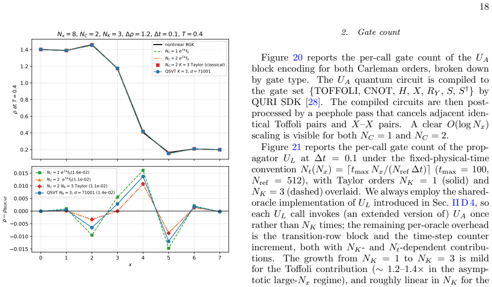
QSVT simulation ofN C = 2case To verify theN C = 2 implementation end-to-end, we run the QSVT circuit atN x = 8,N t = 4,N K = 3,ν= 2, ∆t= 0.1, ∆ρ= 1.2, givingT=N t∆t= 0.4 and the clas- sical nonlinear correction|ρ NC=1 −ρ NC=2|∞ ≈6.1×10 −3 (i.e.≈0.5% of the shock amplitude). The effective condi- tion number isκ eff =λ L/σmin(L)≈7,100 and the QSVT polynomi...
2001
-
[9]
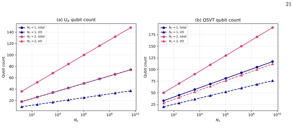
Qubit count Table I summarizes the input/output (I/O) qubit count of each level of the algorithm; the total qubit counts including ancillary qubits are visualised in Fig. 22. Both panels confirm the expected logarithmic growth with the grid sizeN x, with the first-order Carleman im- plementation requiring half as many spatial qubits as the second-order on...
-
[10]
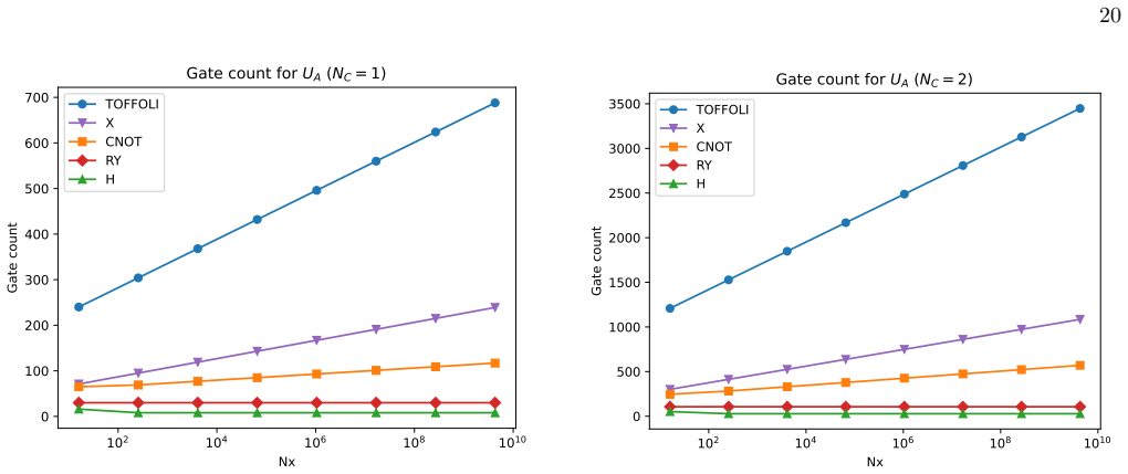
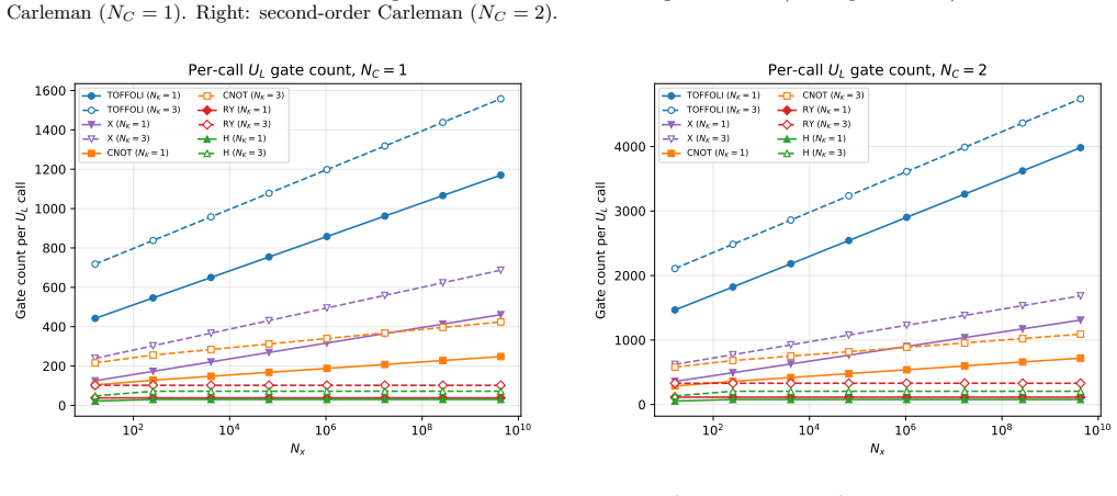
TheU A quantum circuit is compiled to the gate set{TOFFOLI,CNOT, H, X, R Y , S, S †}by QURI SDK [28]
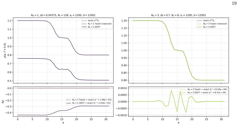
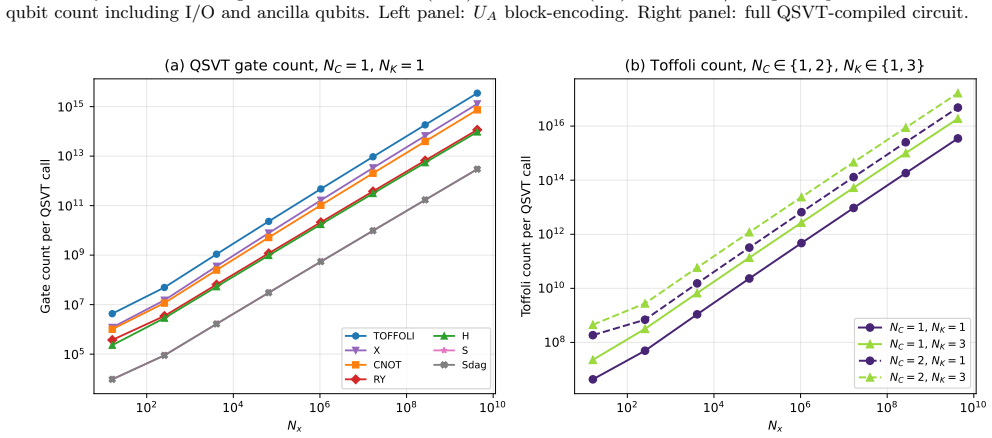
Gate count Figure 20 reports the per-call gate count of theU A block encoding for both Carleman orders, broken down by gate type. TheU A quantum circuit is compiled to the gate set{TOFFOLI,CNOT, H, X, R Y , S, S †}by QURI SDK [28]. The compiled circuits are then post- processed by a peephole pass that cancels adjacent iden- tical Toffoli pairs andX–Xpairs...
-
[11]
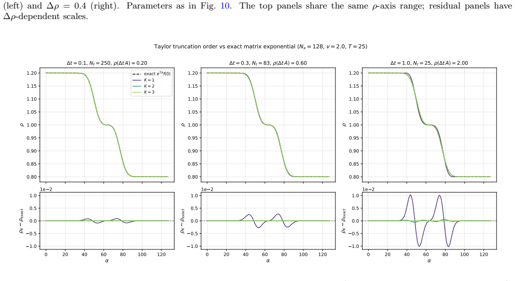
The time axis itself is set by the fixed physical-time conventionN t(Nx) =⌈t max Nx/(Nref ∆tL)⌉(t max = 100, 19 0.5 0.6 0.7 0.8 0.9 1.0 1.1 1.2( , T = 5.6) NK = 1, t = 0.04375, Nt = 128, t = 1200, d = 12001 exact eTAf0 NK = 1 Taylor (classical) NK = 1 QSVT 0.80 0.85 0.90 0.95 1.00 1.05 1.10 1.15 1.20 NK = 3, t = 0.7, Nt = 8, t = 1200, d = 12001 exact eTAf...
2000
-
[12]
Observable extraction and amplitude estimation The QSVT circuit constructed in this work prepares a state|ψ⟩ ∝ |f(T)⟩on the relevant subspace of the solu- tion register, with a success amplitude that scales as 1/κ set by the normalization of the QSP polynomial used to approximate 1/x. Extracting a physical observable such as the drag on a body therefore r...
-
[13]
Higher spatial dimensions and non-trivial geometry The block-encoding construction generalizes to higher spatial dimensions without a qualitative change. AD- dimensional LBM withQvelocity channels andN x grid points per axis requiresD⌈log 2 Nx⌉spatial qubits and ⌈log2 Q⌉velocity qubits per Carleman slot; at orderN C the total qubit count isN C (Dlog 2 Nx ...
-
[14]
Taylor-expanding 1/ρaroundρ 0 = 1, 1 ρ = 1−∆ + ∆ 2 − · · ·,∆ :=ρ−1,(A1) and truncating after the linear term in ∆ gives 1/ρ≈ 2−ρ
Derivation ofA 13 The nonlinearity of the BGK collision enters only throughρu 2 =m 2 1/ρin the equilibrium (2), withm 1 =P j ejfj. Taylor-expanding 1/ρaroundρ 0 = 1, 1 ρ = 1−∆ + ∆ 2 − · · ·,∆ :=ρ−1,(A1) and truncating after the linear term in ∆ gives 1/ρ≈ 2−ρ. Substituting this intoρu 2 yields m2 1 ρ ≈2m 2 1 −m 2 1 ρ,(A2) a sum of a quadratic-in-fleading ...
-
[15]
, whereFandGare the bi- and trilinear maps defined by Eqs
Derivation ofA 23 Differentiatingf (2) =f (1) ⊗f (1) under the full non- linear dynamics gives df(2) dt = ˙f(1) ⊗f (1) +f (1) ⊗ ˙f(1) .(A5) Substituting ˙f(1) =A 11f(1) +F(f (1),f (1)) + G(f(1),f (1),f (1)) +. . ., whereFandGare the bi- and trilinear maps defined by Eqs. (9) and (A4), the right-hand side of Eq. (A5) separates by polynomial degree: degree ...
-
[16]
Under trunca- tion atN C = 3, the couplingsA 34f(4) and higher are dropped
Derivation ofA 33 Repeating the Leibniz argument at rank 3, A33 =A 11 ⊗I⊗I+I⊗A 11 ⊗I+I⊗I⊗A 11,(A10) a Kronecker sum over the three factors. Under trunca- tion atN C = 3, the couplingsA 34f(4) and higher are dropped. The Kronecker-sum structure preserves tensor products, so givenf (3)(0) =f ⊗3 0 the solution is f(3)(t) = etA11 f0 ⊗3 =f (1) lin (t)⊗3,(A11) ...
-
[17]
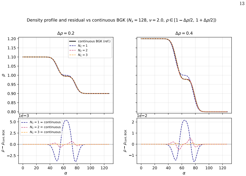
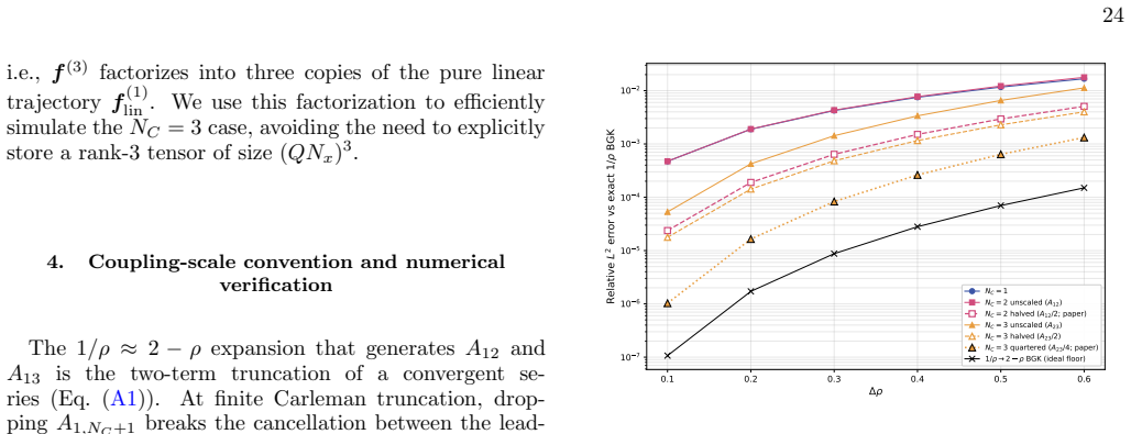
Coupling-scale convention and numerical verification The 1/ρ≈2−ρexpansion that generatesA 12 and A13 is the two-term truncation of a convergent se- ries (Eq. (A1)). At finite Carleman truncation, drop- pingA 1,NC+1 breaks the cancellation between the lead- ing 2m 2 1 in Eq. (A2) and the cubic correction−ρ m 2 1, and the nonlinear source overshoots. To den...
-
[18]
Gaitan, Finding flows of a Navier–Stokes fluid through quantum computing, npj Quantum Information6, 61 (2020)
F. Gaitan, Finding flows of a Navier–Stokes fluid through quantum computing, npj Quantum Information6, 61 (2020)
2020
-
[19]
L. Budinski, Quantum algorithm for the Navier-Stokes equations by using the streamfunction-vorticity for- mulation and the lattice Boltzmann method, Int. J. Quantum Inf.20, 10.1142/s0219749921500398 (2022), arXiv:2103.03804 [quant-ph]
-
[20]
W. Itani and S. Succi, Analysis of Carleman lin- earization of lattice Boltzmann, Fluids7, 24 (2022), arXiv:2111.11327 [quant-ph]
arXiv 2022
-
[21]
X. Li, X. Yin, N. Wiebe, J. Chun, G. K. Schenter, M. S. Cheung, and J. M¨ ulmenst¨ adt, Potential quantum advan- tage for simulation of fluid dynamics, Phys. Rev. Res.7, 013036 (2025), arXiv:2303.16550 [quant-ph]
arXiv 2025
- [22]
-
[23]
M. A. Schalkers and M. M¨ oller, Momentum exchange method for quantum Boltzmann methods, Comput. Flu- ids285, 106453 (2024), arXiv:2404.17618 [quant-ph]
arXiv 2024
-
[24]
D. Jennings, K. Korzekwa, M. Lostaglio, R. Ash- worth, E. Marsili, and S. Rolston, An end-to-end quantum algorithm for nonlinear fluid dynamics with bounded quantum advantage, arXiv [quant-ph] (2025), arXiv:2512.03758 [quant-ph]. Nx τ µ(A),N C =1µ(A),N C =2 ∆t c,N C =1 ∆t c,N C =2 4 0.047 21.3 42.7 0.047 0.023 8 0.094 10.7 21.3 0.094 0.047 16 0.188 5.3 10...
arXiv 2025
-
[25]
D. Jennings, K. Korzekwa, M. Lostaglio, P. Mannix, R. Ashworth, E. Marsili, and S. Rolston, Simulating non-trivial incompressible flows with a quantum lat- tice Boltzmann algorithm, arXiv [quant-ph] (2025), arXiv:2512.05781 [quant-ph]
arXiv 2025
-
[26]
A. D. B. Zamora, B. Ljubomir, L. Valtteri, and S. Pierre, Quantum lattice Boltzmann method for several time steps: A local Carleman linearization algorithm, arXiv [quant-ph] (2025), arXiv:2511.13072 [quant-ph]
arXiv 2025
-
[27]
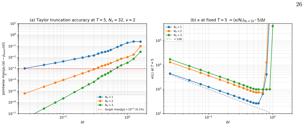
K. Ueno, K. Kanno, and Y. Lee, A demonstration of quantum circuit implementation for obstacle flow using Carleman-linearized lattice Boltzmann method, arXiv:2605.28135 [quant-ph] (2026). 26 10 1 100 t 10 7 10 6 10 5 10 4 10 3 10 2 10 1 100 101 pointwise max| K ( ) exact( )| (a) Taylor truncation accuracy at T = 5, Nx = 32, = 2 NK = 1 NK = 2 NK = 3 target ...
Pith/arXiv arXiv 2026
-
[28]
Y. H. Qian, D. d’Humi` eres, and P. Lallemand, Lattice BGK models for Navier-Stokes equation, Europhys. Lett. 17, 479 (1992)
1992
-
[29]
Chen and G
S. Chen and G. D. Doolen, Lattice Boltzmann method for fluid flows, Annu. Rev. Fluid Mech.30, 329 (1998)
1998
-
[30]
Kruger,The lattice Boltzmann method, 1st ed., Grad- uate texts in physics (Springer International Publishing, Cham, Switzerland, 2016)
T. Kruger,The lattice Boltzmann method, 1st ed., Grad- uate texts in physics (Springer International Publishing, Cham, Switzerland, 2016)
2016
-
[31]
Carleman, Application de la th´ eorie des ´ equations int´ egrales lin´ eaires aux syst` emes d’´ equations diff´ erentielles non lin´ eaires, Acta Math.59, 63 (1932)
T. Carleman, Application de la th´ eorie des ´ equations int´ egrales lin´ eaires aux syst` emes d’´ equations diff´ erentielles non lin´ eaires, Acta Math.59, 63 (1932)
1932
-
[32]
S. K. Leyton and T. J. Osborne, A quantum algo- rithm to solve nonlinear differential equations (2008), arXiv:0812.4423 [quant-ph]
Pith/arXiv arXiv 2008
-
[33]
Joseph, Koopman–von Neumann approach to quantum simulation of nonlinear classical dynamics, Phys
I. Joseph, Koopman–von Neumann approach to quantum simulation of nonlinear classical dynamics, Phys. Rev. Research2, 043102 (2020), arXiv:2003.09980 [quant-ph]
arXiv 2020
-
[34]
J.-P. Liu, H. Ø. Kolden, H. K. Krovi, N. F. Loureiro, K. Trivisa, and A. M. Childs, Efficient quantum al- gorithm for dissipative nonlinear differential equations, Proc. Natl. Acad. Sci. U.S.A.118, e2026805118 (2021), arXiv:2011.03185 [quant-ph]
arXiv 2021
-
[35]
D. W. Berry, A. M. Childs, A. Ostrander, and G. Wang, Quantum algorithm for linear differential equations with exponentially improved dependence on precision, Com- mun. Math. Phys.356, 1057 (2017), arXiv:1701.03684 [quant-ph]
Pith/arXiv arXiv 2017
-
[36]
A. Gily´ en, Y. Su, G. H. Low, and N. Wiebe, Quantum singular value transformation and beyond: exponential improvements for quantum matrix arithmetics, inProc. 51st ACM STOC(2019) pp. 193–204, arXiv:1806.01838 [quant-ph]
arXiv 2019
-
[37]
P. L. Bhatnagar, E. P. Gross, and M. Krook, A model for collision processes in gases. I. small amplitude pro- cesses in charged and neutral one-component systems, Phys. Rev.94, 511 (1954)
1954
-
[38]
G. H. Low and I. L. Chuang, Optimal hamiltonian sim- ulation by quantum signal processing, Phys. Rev. Lett. 118, 010501 (2017), arXiv:1606.02685 [quant-ph]
Pith/arXiv arXiv 2017
-
[39]
D. Aharonov and A. Ta-Shma, Adiabatic quantum state generation and statistical zero knowledge (2003), arXiv:quant-ph/0301023 [quant-ph]
Pith/arXiv arXiv 2003
-
[40]
A. M. Childs,Quantum information processing in contin- uous time, Ph.D. thesis, Massachusetts Institute of Tech- nology (2004)
2004
-
[41]
D. W. Berry, G. Ahokas, R. Cleve, and B. C. Sanders, Efficient quantum algorithms for simulating sparse Hamiltonians, Commun. Math. Phys.270, 359 (2007), arXiv:quant-ph/0508139 [quant-ph]
Pith/arXiv arXiv 2007
-
[42]
D. W. Berry and A. M. Childs, Black-box hamiltonian simulation and unitary implementation, Quantum Inf. Comput.12, 29 (2012), arXiv:0910.4157 [quant-ph]
Pith/arXiv arXiv 2012
-
[43]
S. A. Cuccaro, T. G. Draper, S. A. Kutin, and D. P. Moulton, A new quantum ripple-carry addition cir- cuit, arXiv [quant-ph] (2004), arXiv:quant-ph/0410184 [quant-ph]
Pith/arXiv arXiv 2004
-
[44]
Y. Dong, X. Meng, K. B. Whaley, and L. Lin, Effi- cient phase-factor evaluation in quantum signal process- ing, Phys. Rev. A103, 042419 (2021), arXiv:2002.11649 [quant-ph]
arXiv 2021
-
[45]
com/QunaSys/quri-sdk(2024), accessed: 2026-04-17
QunaSys, QURI SDK: A comprehensive software devel- opment kit for quantum computing,https://github. com/QunaSys/quri-sdk(2024), accessed: 2026-04-17
2024
- [46]
-
[47]
QunaSys, quri-parts-cuquantum: GPU-accelerated state-vector simulation backend for QURI Parts, https://github.com/QunaSys/quri-parts-cuquantum (2024), accessed: 2026-04-17
2024
-
[48]
N. J. Ross and P. Selinger, Optimal ancilla-free Clif- ford+T approximation ofz-rotations, Quantum Infor- mation & Computation16, 901 (2016), arXiv:1403.2975 [quant-ph]
Pith/arXiv arXiv 2016
- [49]
-
[50]
Gribling, I
S. Gribling, I. Kerenidis, and D. Szil´ agyi, An opti- mal linear-combination-of-unitaries-based quantum lin- 27 ear system solver, ACM Trans. Quantum Comput.5, 1 (2024)
2024
-
[51]
G. Brassard, P. Høyer, M. Mosca, and A. Tapp, Quantum amplitude amplification and estimation, Contemp. Math. 305, 53 (2002), arXiv:quant-ph/0005055 [quant-ph]
Pith/arXiv arXiv 2002
-
[52]
A. Ambainis, Variable time amplitude amplification and quantum algorithms for linear systems of equations, in 29th International Symposium on Theoretical Aspects of Computer Science (STACS 2012), Vol. 14 (2012) pp. 636–647, arXiv:1010.4458 [quant-ph]
Pith/arXiv arXiv 2012
-
[53]
P. C. S. Costa, D. An, Y. R. Sanders, Y. Su, R. Bab- bush, and D. W. Berry, Optimal scaling quantum linear- systems solver via discrete adiabatic theorem, PRX Quantum3, 040303 (2022), arXiv:2111.08152 [quant-ph]
arXiv 2022
-
[54]
P. C. S. Costa, A. M. Dalzell, D. An, and D. W. Berry, Constant factor analysis of optimal quantum lin- ear solvers in practice (2026), arXiv:2604.22185 [quant- ph]
Pith/arXiv arXiv 2026
- [55]
-
[56]
M. E. S. Morales, L. Pira, P. Schleich, K. Koor, P. C. S. Costa, D. An, A. Aspuru-Guzik, L. Lin, P. Rebentrost, and D. W. Berry, Quantum linear system solvers: A survey of algorithms and applications, arXiv [quant-ph] (2024), arXiv:2411.02522 [quant-ph]
arXiv 2024
discussion (0)
Sign in with ORCID, Apple, or X to comment. Anyone can read and Pith papers without signing in.