Wave turbulence theory of odd fluids and solids: kinetic equations and solutions
Pith reviewed 2026-06-27 04:35 UTC · model grok-4.3
The pith
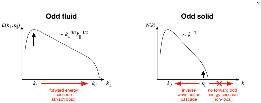
Odd viscosity produces anisotropic Kolmogorov-Zakharov spectra through three-wave interactions while odd elasticity supports a marginally valid inverse cascade of wave action.
A machine-rendered reading of the paper's core claim, the machinery that carries it, and where it could break.
Core claim
In the three-dimensional odd-viscosity model, the wave kinetic equation obtained from three-wave interactions admits a direct-cascade Kolmogorov-Zakharov solution for energy that is anisotropic. In the quasi-one-dimensional odd-elasticity model, the six-wave kinetic equation admits an inverse-cascade Kolmogorov-Zakharov solution for wave action that is only marginally nonlocal (hence physical up to a logarithmic correction) while the corresponding forward-cascade solution for odd energy is nonlocal and unphysical. Both analytical predictions match the spectra seen in direct numerical simulations.
What carries the argument
The wave kinetic equations obtained under the weak-turbulence closure, whose stationary power-law solutions are the Kolmogorov-Zakharov spectra for three-wave (odd viscosity) and six-wave (odd elasticity) interactions.
If this is right
- Direct numerical simulations of odd-viscous fluids must exhibit the anisotropic Kolmogorov-Zakharov spectrum for energy in the direct cascade.
- Direct numerical simulations of odd-elastic solids must exhibit the marginally nonlocal Kolmogorov-Zakharov spectrum for wave action in the inverse cascade.
- The forward cascade of odd energy is ruled out as a physical steady state in the odd-elasticity model.
- The distinction between three-wave and six-wave regimes is fixed by the dispersion relation and the breaking of time-reversal symmetry in each model.
Where Pith is reading between the lines
- The same kinetic-equation approach could be applied to other chiral or non-reciprocal media whose dispersion relations similarly select three-wave or six-wave resonances.
- The logarithmic correction required for the inverse cascade suggests that finite-size or forcing-scale effects may shift the observed exponent in simulations or experiments of odd-elastic systems.
- The anisotropy of the odd-viscosity spectrum implies that energy transfer rates differ along versus perpendicular to the preferred direction set by the odd stress.
Load-bearing premise
The simple models for odd viscosity and odd elasticity permit the interaction order to be fixed by the dispersion relations and symmetry properties so that the closed-form kinetic equations capture the dominant dynamics.
What would settle it
A direct numerical simulation of the three-dimensional odd-viscosity model whose energy spectrum deviates from the predicted anisotropic Kolmogorov-Zakharov scaling in the inertial range would falsify the three-wave theory.
Figures
read the original abstract
The theory of wave turbulence describes the properties of physical systems composed of a set of weak-amplitude random waves interacting nonlinearly. Here, we study odd wave turbulence, which arises in chiral media subjected to non-reciprocal stresses, notably odd viscosity and odd elasticity. In both cases, we consider simple models for which we can derive and solve analytically the kinetic equations describing the long-term statistical behavior of spectral quantities such as energy or wave action. For odd viscosity, we consider a three-dimensional model that exhibits wave turbulence involving three-wave interactions, which gives rise to a direct energy cascade characterized by an anisotropic Kolmogorov-Zakharov (KZ) spectrum. For odd elasticity, we consider a quasi-one-dimensional overdamped model that exhibits much slower dynamics involving six-wave interactions. In that case, the KZ spectrum corresponding to a forward cascade of a conserved quantity we call odd energy, is nonlocal and therefore does not constitute a physical solution. However, the other KZ solution, which describes an inverse cascade of wave action, is only marginally non-local and is therefore valid up to a logarithmic correction. These two analytical theories provide a rigorous interpretation of direct numerical simulations, where the KZ spectrum is observed both in the case of odd viscosity (forward cascade) and of odd elasticity (inverse cascade).
Editorial analysis
A structured set of objections, weighed in public.
Referee Report
Summary. The paper develops wave-turbulence kinetic theory for chiral media with non-reciprocal stresses. For a 3D model with odd viscosity it derives a three-wave kinetic equation whose stationary solutions include an anisotropic Kolmogorov-Zakharov spectrum describing a direct energy cascade. For a quasi-1D overdamped model with odd elasticity it derives a six-wave kinetic equation; the forward-cascade solution for a conserved quantity termed “odd energy” is shown to be nonlocal and unphysical, while the inverse-cascade solution for wave action is only marginally nonlocal and therefore admissible up to a logarithmic correction. Both spectra are reported to be consistent with direct numerical simulations.
Significance. If the derivations and locality assessments hold, the work supplies the first analytic wave-turbulence description of odd-viscous and odd-elastic systems, furnishing explicit, falsifiable KZ spectra that interpret existing simulations. The explicit construction of the interaction coefficients, the order counting that fixes three-wave versus six-wave dynamics, and the locality analysis constitute the principal technical contributions.
minor comments (3)
- §2.2: the resonance manifold for the three-wave process is stated but the explicit form of the interaction coefficient T_{1,2,3} is not written out; including it would allow direct verification of the matrix-element symmetries used later.
- Eq. (37): the logarithmic correction to the inverse-cascade spectrum is asserted but the precise range of wavenumbers over which the marginal non-locality remains tolerable is not quantified; a short estimate or plot would strengthen the claim.
- Figure 4 caption: the DNS spectra are overlaid on the analytic KZ prediction, yet the fitting procedure (e.g., choice of prefactor, range of k used) is not described; this detail is needed for reproducibility.
Simulated Author's Rebuttal
We thank the referee for their positive assessment of our manuscript and for recommending minor revision. The referee's summary correctly captures the scope and main findings of the work on odd wave turbulence.
Circularity Check
No significant circularity: standard weak-turbulence derivation applied to new dispersion relations
full rationale
The paper selects simple models of odd viscosity (3D, three-wave) and odd elasticity (quasi-1D overdamped, six-wave) precisely because their dispersion relations and symmetries permit closed analytic kinetic equations under the standard weak-turbulence closure. The Kolmogorov-Zakharov spectra are then obtained by the usual Zakharov transformation and locality analysis; none of these steps reduce the final spectra or cascade directions to quantities fitted inside the paper or to self-citations whose validity depends on the present work. The derivation chain is therefore self-contained against external benchmarks of wave-turbulence theory.
Axiom & Free-Parameter Ledger
axioms (2)
- domain assumption Weak-amplitude random waves interacting nonlinearly under the wave-turbulence closure
- domain assumption Dispersion relations of the chosen odd-viscosity and odd-elasticity models fix the interaction order at three or six waves
invented entities (1)
-
odd energy
no independent evidence
Reference graph
Works this paper leans on
-
[1]
Detailed conservation laws The kinetic equation satisfies the conservation of energy and helicity. To prove this property, we introduce the energy spectrum E(k) =e +(k) +e −(k) = X s es(k)(42) and the helicity spectrum H(k) =k ⊥(e+(k)−e −(k)) =k ⊥ X s ses(k).(43) For the energy, we find ∂ R E(k)dk ∂t = πϵ2 16 X sspsq Z k∥ sinθ k k⊥ 2 spp⊥ −s qq⊥ k∥ 2 (44)...
-
[2]
Kolmogorov-Zakharov spectrum The derivation of the stationary solutions requires a long but classical calculation. First, we assume axisymmetry and introduce the reduced spectrum Es k ≡E s(k⊥, k∥) = 2πk⊥es(k).(48) The kinetic equation (39) now reads ∂E s k ∂t = ϵ2k∥ 32νodd X spsq Z sin2 θk k⊥ 1 k⊥p⊥q⊥ spp⊥ −s qq⊥ k∥ 2 (sk⊥ +s pp⊥ +s qq⊥)2 (49) × ωkEsp p E...
-
[3]
Let us now integrate this equation with respect tok⊥ on the one hand, andk∥ on the other hand
Cascade direction We now introduce the axisymmetric energy flux, ∂tEk =− ∂Π⊥(k⊥, k∥) ∂k⊥ − ∂Π∥(k⊥, k∥) ∂k∥ .(62) From the kinetic equation (59), we write ∂tEk = ϵ2A2 384νodd k2n+2 ⊥ k2m ∥ I(n, m),(63) 11 whereI(n, m)is the normalized collisional integral. Let us now integrate this equation with respect tok⊥ on the one hand, andk∥ on the other hand. Taking...
-
[4]
This ratio decreases as we go towards the small scales
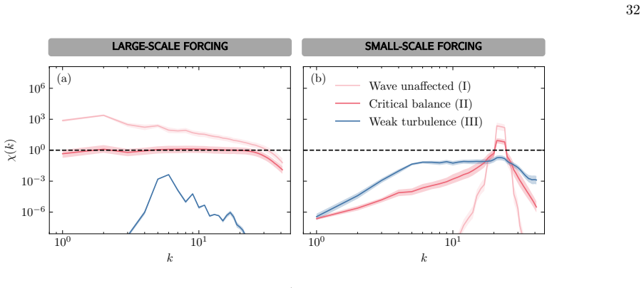
Validity of the weak wave regime and inertial range As mentioned at the beginning of this section, the range of validity of weak wave turbulence theory can be estimated by evaluating the ratio of the linear timescaleτlin ∼ω −1 k and the non-linear time scale estimated from the equation of motion (1),τ NL ∼1/(kv)∼1/(k p k⊥k∥E(k⊥, k∥)), χ≡ τlin τNL ∼ p k⊥k∥...
-
[5]
Introduction of the model In this second part of the paper, we study the propagation of one-dimensional nonlinear shear waves in incompressible chiral active solids. The evolution of the displacement fieldu(t, z)(wherezis the direction of propagation) is given by ρ0∂2 t u+ Γ∂ tu=∇·σ(72) in whichσis the stress tensor andρ 0 is the density of the unperturbe...
-
[6]
At the linear level, Eq
Overdamped limit and wave propagation In order to allow for the propagation of waves, we consider the overdamped limit, ∂tu= (G+G oddϵ)∂2 z u+ (G NL +G NL oddϵ)∂z ∥∂zu∥2∂zu +g(75) in which we introduceGi =µ i/Γfor each of the four elastic moduli, andg=f/Γ. At the linear level, Eq. (75) admits wave-like solutions. Substitution of a solution of the formexp(...
-
[7]
However, in the present case, the ratio of the dissipation timescale τdiss ∼1/(Gk 2)due to shear elasticity with the linear timescaleτlin ∼ω −1 ∼1/(G oddk2)is independent ofk
Shear elasticity and dissipation An important requirement for the application of weak wave turbulence theory is the existence of an inertial range where forcing and dissipation are negligible. However, in the present case, the ratio of the dissipation timescale τdiss ∼1/(Gk 2)due to shear elasticity with the linear timescaleτlin ∼ω −1 ∼1/(G oddk2)is indep...
-
[8]
Below we give an example of a microscopic model which reduces to Eq
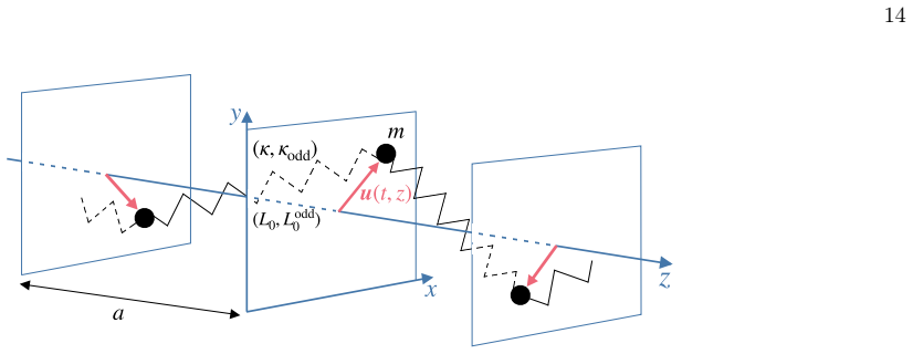
Possible experimental realizations Equation (74) has been obtained from symmetry. Below we give an example of a microscopic model which reduces to Eq. (74) upon coarse-graining, namely a one-dimensional chain where particles confined in fixedzplanes and free to move within the plane are connected to their neighbors by both normal and odd springs, with a r...
-
[9]
Derivation from a microscopic model The equation (74) can be obtained by taking the continuous limit of a microscopic model, such as the one depicted in Fig. 2. Consider a chain of particles of massm. Each particle is constrained to move inside a plane(x, y)orthogonal to the directionzof the chain. Two neighboring planes are separated by a distancea. Neig...
-
[10]
A simple model of odd elastic solid In the remainder of the paper, we focus on the model of a one-dimensional shear-wave odd elastic solid constructed in Sec. IIIA where the deformation fieldu(t,r)follows ∂tu=G oddϵ∂2 z u+G NL oddϵ∂z ∥∂zu∥2∂zu +D+g(90) whereDdescribes the dissipation of wave action and odd energy, whilegis a stochastic driving force. We r...
-
[11]
This is where the main difference between odd viscous fluids and odd elastic solids arises
Equation in canonical form and conserved quantities The existence of waves which interact via a weak non-linearity is not the only ingredient required for the development of wave turbulence: it also requires the existence of one or several conserved quantities which can cascade through scales. This is where the main difference between odd viscous fluids a...
-
[12]
Focusing on the limit of weak non-linearity, i.e.GNL odd ≪G odd, we can therefore apply the framework of weak wave turbulence theory to our system
Wave turbulence phenomenology and overview We have now shown that our model possesses all the ingredients for wave turbulence: (i) the existence of wave-like solutions that are subject to a weak non-linear interaction, and (ii) several conserved quantities, which in this case are emergent quantities specific to this system. Focusing on the limit of weak n...
-
[13]
The idea is to perform a change of variable fromA(t, k)to a new variablec(t, k)
Canonical transformation In this subsection, we derive the coefficient of the six-wave interaction following the same approach as [1, 77–80]. The idea is to perform a change of variable fromA(t, k)to a new variablec(t, k). This change of variable should be canonical, i.e. it should conserve the Hamilton equation (100). For this, we take advantage of the f...
-
[14]
To leading order we still have n(k)δ(k−k ′) =⟨c kc∗ k′⟩.(123) We start from equation (122)
Wave kinetic equation We now derive the kinetic equation for the wave action spectrumn(k), following the random phase approximation method as presented in [1]. To leading order we still have n(k)δ(k−k ′) =⟨c kc∗ k′⟩.(123) We start from equation (122). Multiplying this equation byc ∗ k′, subtracting the complex conjugate withk↔k ′, averaging and multiplyin...
-
[15]
Detailed conservation laws Introducing the quantity Φ = Z dkρknk ,(129) and using the kinetic equation (128), we can write after symmetrization ∂tΦ = Z dkρk∂tnk (130) = π 36 Z k12345 (W345 k12)2nkn1n2n3n4n5 1 nk + 1 n1 + 1 n2 − 1 n3 − 1 n4 − 1 n5 [ρk +ρ 1 +ρ 2 −ρ 3 −ρ 4 −ρ 5] ×δ(k+k 1 +k 2 −k 3 −k 4 −k 5)δ(ωk +ω 1 +ω 2 −ω 3 −ω 4 −ω 5). 22 From this expres...
-
[16]
From here on, we assume that the spectrum is even ink,n(k) =n(−k)
Zakharov-Kolmogorov spectra We now look for stationary solutions of the kinetic equation (128) using the Kuznetsov-Zakharov transformation [1]. From here on, we assume that the spectrum is even ink,n(k) =n(−k). This implies thatN(k) =n(k)in (106), and that the odd momentumPvanishes. Let us introduce, fork∈R +, the functionf(k)such that f(k) =ω k =|G odd|k...
-
[17]
Nature of the cascades Let us now consider the kinetic equation (128) withn(k) =N(k) =C|k| −ν and rescale the integral to take out all thekdependence by writingk i =kz i fori= 1,2,3,4,5. This gives ∂tNk = (GNL odd)4 |Godd|3 C5k14−5νI(ν),(156) where I(ν) = π 6 Z dz1dz2dz3dz4dz5 (wz3z4z5 1z1z2 )2(z1z2z3z4z5)−ν [1 +z ν 1 +z ν 2 −z ν 3 −z ν 4 −z ν 5 ] ×δ(1 +z...
-
[18]
This is called the locality hypothesis
Locality of the interaction For the above solutions to be valid, the collision integral in the kinetic wave equation (128) needs to converge. This is called the locality hypothesis. If the integral diverges for a given KZ solution, then this solution cannot be realized. For this section it is convenient to integrate over the two delta functions, leading t...
-
[19]
We write ΠN(k) = Z k dk∂tNk ∝ Z k dk k14N5 k ∝ Z k dk k−1 ln−5y(kℓd).(175) This integrates to some power ofln(kℓd), except fory= 1/5for which we obtainΠ N(k)∝ln ln(kℓ d)
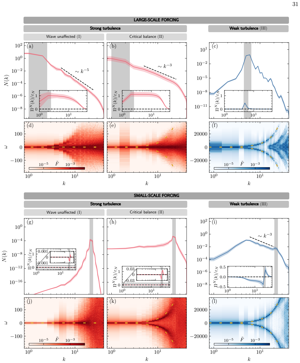
Logarithmic correction Following the argument of [78] (first developed by Kraichnan for 2D eddy turbulence [81]), we assume that the spectrum for the wave action cascade can be corrected as N(k) =C N |Godd|3/5|GNL odd|−4/5ε1/5 N k−3 ln−y(kℓd),(174) whereℓ d is the scale at which large scale dissipation occurs. We write ΠN(k) = Z k dk∂tNk ∝ Z k dk k14N5 k ...
-
[20]
We recall that the integralI(ν)vanishes forν= 3, since this is a stationary solution of the kinetic equation
DAM approximation and direction of the cascades Let us now finally investigate the direction of the cascade. We recall that the integralI(ν)vanishes forν= 3, since this is a stationary solution of the kinetic equation. However the denominator in (160) also vanishes at this value. Thus, in this case the wave action flux reads instead (omitting the logarith...
-
[21]
Beyond the weak wave regime Let us now estimate the domain of validity of our weak wave turbulence prediction. From the kinetic equation (128), we can evaluate the transfer time of the wave action cascade, τtr ∼ (GNL odd)4 G3 odd k14N(k) 4 −1 .(194) Note that the wave action flux can be estimated from this transfer time as ΠN ∼ kN(k) τtr ∼ (GNL odd)4 G3 o...
-
[22]
Numerical implementation In order to test the theoretical predictions, we numerically simulate our toy model for the odd elastic solid, probing the different strong and weak states. To enter into a driven-dissipative state analogous to fully developed turbulence, we include a stochastic forcing (gin equation (90)) that injects energy through additive Gaus...
-
[23]
N ª k °3 (b) 10 0 10 1 0 1 ¶ N (k)/
Results The results are provided in Fig. 4. This shows the time-averaged and spatio-temporal spectra of the wave action N(k), as well as the fluxΠN(k)thereof. Note that the flux can be obtained in the standard way from the inner product between the amplitudeuand the non-linear term in Fourier space. We find that in the strong regime, two distinct behavior...
2023
-
[24]
Zakharov, V
V. Zakharov, V. L’Vov, and G. Falkovich,Kolmogorov spectra of turbulence I: Wave turbulence(Springer Series in Nonlinear Dynamics, Berlin: Springer, 1992, 1992)
1992
-
[25]
Nazarenko,Wave Turbulence, Lecture Notes in Physics, Vol
S. Nazarenko,Wave Turbulence, Lecture Notes in Physics, Vol. 825 (Berlin Springer Verlag, 2011)
2011
-
[26]
A. C. Newell and B. Rumpf, Annu. Rev. Fluid Mech.43, 59–78 (2011)
2011
-
[27]
Galtier,Physics of Wave Turbulence(Cambridge University Press, 2023)
S. Galtier,Physics of Wave Turbulence(Cambridge University Press, 2023)
2023
-
[28]
Fruchart, C
M. Fruchart, C. Scheibner, and V. Vitelli, Annu. Rev. Condens. Matter Phys.14, 471–510 (2023)
2023
-
[29]
A.I.Berdyugin, S.G.Xu, F.M.D.Pellegrino, R.K.Kumar, A.Principi, I.Torre, M.B.Shalom, T.Taniguchi, K.Watanabe, I. V. Grigorieva, M. Polini, A. K. Geim, and D. A. Bandurin, Science364, 162–165 (2019)
2019
-
[30]
V. Soni, E. S. Bililign, S. Magkiriadou, S. Sacanna, D. Bartolo, M. J. Shelley, and W. T. M. Irvine, Nat. Phys.15, 1188–1194 (2019)
2019
-
[31]
J. J. M. Beenakker and F. R. McCourt, Annu. Rev. Phys. Chem.21, 47–72 (1970)
1970
-
[32]
W. M. Stacey, R. W. Johnson, and J. Mandrekas, Physics of Plasmas13, 062508 (2006)
2006
-
[33]
C. Bae, W. Stacey, and W. Solomon, Nuclear Fusion53, 043011 (2013)
2013
-
[34]
Kono and J
M. Kono and J. Vranjes, Physics of Plasmas22, 112101 (2015)
2015
-
[35]
Scheibner, A
C. Scheibner, A. Souslov, D. Banerjee, P. Surówka, W. T. M. Irvine, and V. Vitelli, Nat. Phys.16, 475–480 (2020)
2020
-
[36]
Y. Chen, X. Li, C. Scheibner, V. Vitelli, and G. Huang, Nature Communications12, 10.1038/s41467-021-26034-z (2021)
-
[37]
Veenstra, C
J. Veenstra, C. Scheibner, M. Brandenbourger, J. Binysh, A. Souslov, V. Vitelli, and C. Coulais, Nature639, 935–941 (2025)
2025
-
[38]
E. S. Bililign, F. Balboa Usabiaga, Y. A. Ganan, A. Poncet, V. Soni, S. Magkiriadou, M. J. Shelley, D. Bartolo, and W. T. M. Irvine, Nature Physics18, 212–218 (2021)
2021
-
[39]
T. H. Tan, A. Mietke, J. Li, Y. Chen, H. Higinbotham, P. J. Foster, S. Gokhale, J. Dunkel, and N. Fakhri, Nature607, 287–293 (2022)
2022
-
[40]
Y.-C. Chao, S. Gokhale, L. Lin, A. Hastewell, A. Bacanu, Y. Chen, J. Li, J. Liu, H. Lee, J. Dunkel, and N. Fakhri, Nature Physics22, 474–482 (2026)
2026
-
[41]
Shankar and L
S. Shankar and L. Mahadevan, Nature Physics20, 1501–1508 (2024)
2024
- [42]
-
[43]
Benney and P
D. Benney and P. Saffman, Proc. R. Soc. Lond. A289, 301–320 (1966)
1966
-
[44]
Newell, Rev
A. Newell, Rev. Geophys.6, 1–31 (1968)
1968
-
[45]
Galtier, C
S. Galtier, C. R. Phys.25, 433–455 (2024)
2024
-
[46]
Zakharov and N
V. Zakharov and N. Filonenko, J. Applied Mech. Tech. Phys.8, 37 (1967)
1967
-
[47]
Yarom and E
E. Yarom and E. Sharon, Nat. Phys.10, 510 (2014)
2014
-
[48]
Galtier and S
S. Galtier and S. Nazarenko, Phys. Rev. Lett.119, 221101 (2017)
2017
-
[49]
Düring, C
G. Düring, C. Josserand, and S. Rica, Phys. D: Nonlinear Phenom.347, 42–73 (2017)
2017
-
[50]
Meyrand, K
R. Meyrand, K. Kiyani, O. Gürcan, and S. Galtier, Phys. Rev. X8, 031066 (2018)
2018
-
[51]
Hassaini, N
R. Hassaini, N. Mordant, B. Miquel, G. Krstulovic, and G. Düring, Phys. Rev. E99, 033002 (2019)
2019
-
[52]
Le Reun, B
T. Le Reun, B. Favier, and M. Le Bars, Europhys. Lett.132, 64002 (2020)
2020
-
[53]
Monsalve, M
E. Monsalve, M. Brunet, B. Gallet, and P.-P. Cortet, Phys. Rev. Lett.125, 254502 (2020)
2020
-
[54]
Galtier and S
S. Galtier and S. Nazarenko, Phys. Rev. Lett.127, 131101 (2021)
2021
-
[55]
Ricard and E
G. Ricard and E. Falcon, EPL (Europhysics Letters)135, 64001 (2021)
2021
-
[56]
Falcon and N
E. Falcon and N. Mordant, Ann. Rev. Fluid Mech.54, 1 (2022)
2022
-
[57]
Griffin, G
A. Griffin, G. Krstulovic, V. L’vov, and S. Nazarenko, Phys. Rev. Lett.128, 224501 (2022)
2022
-
[58]
Rodda, C
C. Rodda, C. Savaro, G. Davis, J. Reneuve, P. Augier, J. Sommeria, T. Valran, S. Viboud, and N. Mordant, Phys. Rev. Fluids7, 094802 (2022)
2022
-
[59]
David, S
V. David, S. Galtier, and R. Meyrand, Phys. Rev. Lett.132, 085201 (2024)
2024
-
[60]
E. A. Kochurin and E. A. Kuznetsov, Phys. Rev. Lett.133, 207201 (2024)
2024
-
[61]
S. Zhao, H. Yan, T. Z. Liu, K. H. Yuen, and H. Wang, Nature Astronomy8, 725 (2024)
2024
-
[62]
Khain, C
T. Khain, C. Scheibner, M. Fruchart, and V. Vitelli, J. Fluid Mech.934, A23 (2022)
2022
-
[63]
Avron, J
J. Avron, J. Stat. Phys.92, 543–557 (1998)
1998
-
[64]
X. M. de Wit, M. Fruchart, T. Khain, F. Toschi, and V. Vitelli, Nature627, 515–521 (2024)
2024
-
[65]
S. Chen, X. M. de Wit, M. Fruchart, F. Toschi, and V. Vitelli, Phys. Rev. Lett.133, 144002 (2024)
2024
-
[66]
J. C. Higdon, Astrophys. J.285, 109 (1984)
1984
-
[67]
Goldreich and S
P. Goldreich and S. Sridhar, Astrophys. J.438, 763 (1995)
1995
-
[68]
S. V. Nazarenko and A. A. Schekochihin, J. Fluid Mech.677, 134–153 (2011)
2011
-
[69]
Oughton and W
S. Oughton and W. H. Matthaeus, Astrophys. J.897, 37 (2020)
2020
-
[70]
Zhou, Phys
Y. Zhou, Phys. Rep.935, 1–117 (2021)
2021
-
[71]
Alexakis and L
A. Alexakis and L. Biferale, Phys. Rep.767–769, 1–101 (2018)
2018
-
[72]
Shaltiel, A
O. Shaltiel, A. Salhov, O. Gat, and E. Sharon, Phys. Rev. Lett.132, 224001 (2024)
2024
-
[73]
Galtier, J
S. Galtier, J. Fluid Mech.974, A24 (2023)
2023
-
[74]
R. H. Kraichnan, J. Fluid Mech.59, 745–752 (1973). 35
1973
-
[75]
Waleffe, Phys
F. Waleffe, Phys. Fluids A4, 350–363 (1992)
1992
-
[76]
Turner, J
L. Turner, J. Fluid Mech.408, 205–238 (2000)
2000
-
[77]
Galtier, Phys
S. Galtier, Phys. Rev. E68, 015301 (2003)
2003
-
[78]
Galtier, J
S. Galtier, J. Plasma Phys.72, 721–769 (2006)
2006
-
[79]
Galtier, J
S. Galtier, J. Fluid Mech.757, 114–154 (2014)
2014
-
[80]
Nazarenko and A
S. Nazarenko and A. Schekochihin, J. Fluid Mech.677, 134 (2011)
2011
discussion (0)
Sign in with ORCID, Apple, or X to comment. Anyone can read and Pith papers without signing in.