Structure-Aware Variance Reduction for Unbiased Randomized Hamiltonian Simulation
Pith reviewed 2026-06-26 08:20 UTC · model grok-4.3
The pith
Continuous TE-PAI removes Trotter discretization error with finite-depth random circuits while structure-aware variance reduction cuts sampling costs by 91-96%.
A machine-rendered reading of the paper's core claim, the machinery that carries it, and where it could break.
Core claim
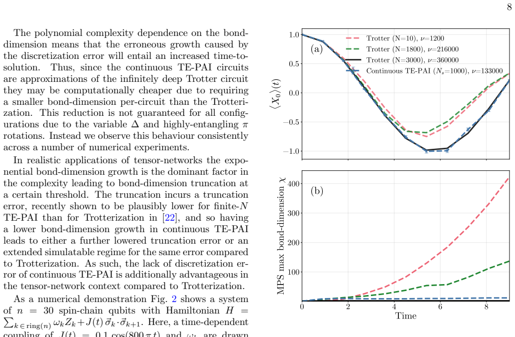
Continuous TE-PAI is a quasiprobabilistic random-circuit protocol whose remaining Monte Carlo error is purely statistical. It removes Trotter discretization error with finite-depth random circuits, whereas deterministic Trotterization requires the infinite-depth limit. The variance of randomized product-formula-based estimators admits a canonical decomposition into a classical counting component and a quantum ordering component such that the dominant simulation overhead results from the non-commutative parts of the Hamiltonian dynamics. Structure-aware variance reduction applied to the counting component yields approximately 70% error reduction for small systems and 80% for n=30 spin-chain d
What carries the argument
continuous time-evolution probabilistic angle interpolation (continuous TE-PAI), a quasiprobabilistic random-circuit protocol that interpolates evolution angles continuously to produce unbiased estimators
If this is right
- Finite-depth random circuits suffice to eliminate discretization error where deterministic methods require infinite depth.
- Tensor-network simulations of continuous TE-PAI circuits avoid the unphysical exponential growth in bond dimension that appears under Trotterization.
- Coarser statistics tailored to the observable and estimator can still produce negligible bias while cutting sampling cost.
- The counting-component reduction applies directly to observable estimation on spin-chain dynamics.
Where Pith is reading between the lines
- The variance decomposition may allow similar counting-focused reductions in other quasiprobabilistic simulation protocols that use product formulas.
- The finite-depth unbiased property could be tested on hardware by comparing expectation values from short random circuits against exact diagonalization on small systems.
- Avoiding bond-dimension blow-up suggests continuous TE-PAI may remain tractable for tensor-network methods on longer chains or higher-dimensional lattices where Trotterization fails.
- The approach leaves open whether ordering-component variance can be further suppressed by additional classical post-processing.
Load-bearing premise
The variance of randomized product-formula estimators admits a decomposition into a classical counting component and a quantum ordering component with the counting component carrying the dominant overhead.
What would settle it
Direct verification that the mean channel of a finite-depth continuous TE-PAI circuit deviates from the exact time-evolution operator, or tensor-network simulations in which continuous TE-PAI circuits exhibit the same exponential bond-dimension growth seen in Trotterized circuits.
Figures
read the original abstract
Randomized Hamiltonian simulation methods are often governed by a trade-off between systematic bias and sampling overhead. We study how classical variance-reduction techniques can be applied to such methods without changing their mean channel, and therefore without introducing additional bias. As a motivating unbiased estimator, we formulate continuous time-evolution probabilistic angle interpolation (continuous TE-PAI), a quasiprobabilistic random-circuit protocol whose remaining Monte Carlo error is purely statistical. Continuous TE-PAI removes Trotter discretization error with finite-depth random circuits, whereas deterministic Trotterization does so only in the infinite-depth limit. Further, in tensor-network simulations, we demonstrate that discretization error can cause an unphysical exponential growth in the bond dimension required for Trotterized simulations, whereas comparable-depth continuous TE-PAI circuits avoid this growth. We then show that the variance of randomized product-formula-based estimators admits a canonical decomposition into a classical counting component and a quantum ordering component such that the dominant simulation overhead results from the non-commutative parts of the Hamiltonian dynamics. Motivated by this decomposition, we achieve an $\approx70\%$ error-reduction using the counting-component for small systems whereas our tensor-network simulations of $n=30$ spin-chain dynamics use coarser statistics tailored to the observable and estimator attaining a negligible bias and a reduction of $\approx 80\%$ leading to $\approx91\%$ and $\approx96\%$ sampling-cost reductions, respectively.
Editorial analysis
A structured set of objections, weighed in public.
Referee Report
Summary. The paper introduces continuous time-evolution probabilistic angle interpolation (continuous TE-PAI) as an unbiased quasiprobabilistic random-circuit protocol for Hamiltonian simulation. It claims that this method removes Trotter discretization error in expectation using finite-depth circuits (unlike deterministic Trotterization, which requires the infinite-depth limit), demonstrates via tensor networks that discretization can induce unphysical exponential bond-dimension growth while continuous TE-PAI avoids it, and shows that the variance of randomized product-formula estimators decomposes canonically into a classical counting component and a quantum ordering component. Structure-aware variance reduction on the counting component is reported to yield ~70% error reduction for small systems and ~80% for n=30 spin chains, with corresponding sampling-cost reductions of ~91% and ~96%.
Significance. If the unbiasedness and variance decomposition hold, the work offers a route to bias-free randomized simulation with reduced Monte Carlo overhead, particularly when the counting component dominates due to non-commutativity. The tensor-network evidence on bond-dimension behavior and the reported cost reductions would be practically relevant for near-term simulation of spin-chain dynamics. The explicit decomposition into counting and ordering components is a clear conceptual contribution that could guide further variance-reduction techniques.
minor comments (3)
- The abstract states specific numerical improvements (~70%, ~80%, ~91%, ~96%) from tensor-network simulations; the main text should include the precise observable choices, data-exclusion criteria, and error-bar reporting to allow verification that the reductions are not post-hoc.
- Notation for the continuous TE-PAI protocol and the counting/ordering variance split should be introduced with explicit equations early in the methods section so that later claims about preservation of the mean channel can be traced directly.
- The tensor-network bond-dimension comparison would benefit from a supplementary figure showing the growth rate versus depth for both methods on the same Hamiltonian instance.
Simulated Author's Rebuttal
We thank the referee for their positive assessment of the manuscript, including the recognition of the unbiasedness property, the variance decomposition, the tensor-network evidence on bond-dimension behavior, and the reported sampling-cost reductions. The recommendation for minor revision is noted. No specific major comments appear in the provided report, so we have no individual points requiring rebuttal or clarification at this stage. We remain available to address any additional comments or to implement minor revisions as directed by the editor.
Circularity Check
No significant circularity; derivation self-contained
full rationale
The paper formulates continuous TE-PAI as an unbiased quasiprobabilistic estimator and derives a variance decomposition into counting and ordering components from the structure of randomized product formulas. These steps are presented as explicit constructions and demonstrations (including tensor-network simulations for n=30 chains) rather than reductions to fitted parameters or self-citations. No load-bearing claim reduces by the paper's equations to a quantity defined in terms of itself, and the reported error reductions are empirical outcomes of applying the decomposition, not forced by construction. The central unbiasedness and variance claims remain independent of the variance-reduction technique.
Axiom & Free-Parameter Ledger
invented entities (1)
-
continuous TE-PAI
no independent evidence
Reference graph
Works this paper leans on
-
[1]
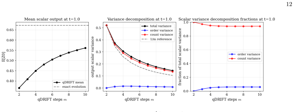
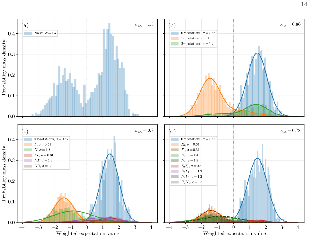
sign-aware, so that quasiprobability signs are fixed within strata; 12 FIG. 4. A small qDRIFT example on the 2-qubit HamiltonianH= 1 2(X0 +X 1) +Z 0Z1 att= 1, varying the qDRIFT step numberm, and estimating⟨Z 0⟩. The left panel shows convergence of the qDRIFT mean to the exact value. The middle panel shows the scalar trajectory-variance decomposition into...
-
[2]
local or observable-adapted, so that they focus on gates visible to the measured observable
-
[3]
Thus the counts-vector theory supplies the ideal abelian reference point, while the numerical TE-PAI procedures use scalable approximations to that reference
small enough that conditional sampling and finite- budget allocation remain practical. Thus the counts-vector theory supplies the ideal abelian reference point, while the numerical TE-PAI procedures use scalable approximations to that reference. V. NUMERICAL SIMULATION In this work we do not aim to determine the opti- mal variance-reduction protocol for u...
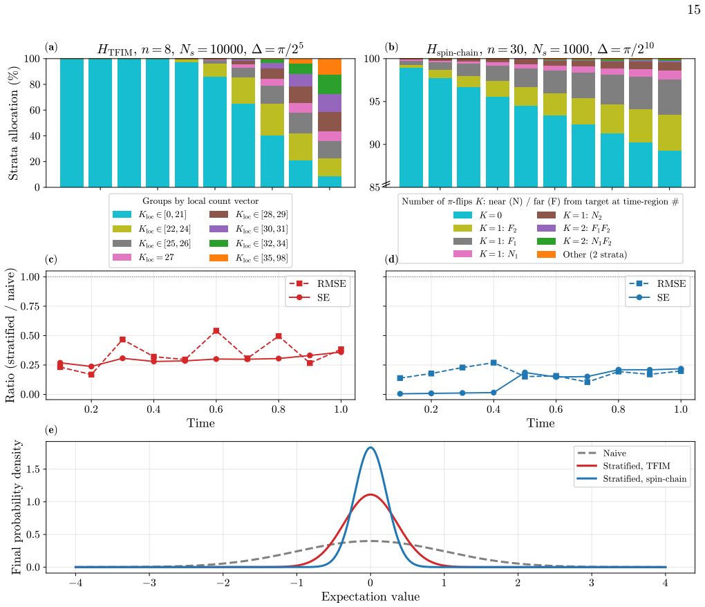
-
[4]
R. P. Feynman, Simulating physics with computers, In- ternational Journal of Theoretical Physics21, 467–488 (1982)
1982
-
[5]
Lloyd, Universal quantum simulators, Science273, 1073–1078 (1996)
S. Lloyd, Universal quantum simulators, Science273, 1073–1078 (1996)
1996
-
[6]
A. M. Childs and N. Wiebe, Hamiltonian simulation us- ing linear combinations of unitary operations, Quantum Information and Computation12, 901–924 (2012)
2012
-
[7]
D. W. Berry, A. M. Childs, R. Cleve, R. Kothari, and R. D. Somma, Exponential improvement in precision for simulating sparse hamiltonians, inProceedings of the forty-sixth annual ACM symposium on Theory of com- puting, STOC ’14 (ACM, 2014)
2014
-
[8]
D. W. Berry, A. M. Childs, R. Cleve, R. Kothari, and R. D. Somma, Simulating hamiltonian dynamics with a truncated taylor series, Physical Review Letters114, 10.1103/physrevlett.114.090502 (2015)
-
[9]
G. H. Low and I. L. Chuang, Optimal hamiltonian sim- ulation by quantum signal processing, Physical Review Letters118, 10.1103/physrevlett.118.010501 (2017)
-
[10]
G. H. Low and I. L. Chuang, Hamiltonian simulation by qubitization, Quantum3, 163 (2019)
2019
-
[11]
A. M. Childs, A. Ostrander, and Y. Su, Faster quantum simulation by randomization, Quantum3, 182 (2019)
2019
-
[12]
Campbell, Random compiler for fast hamiltonian sim- ulation, Physical Review Letters123, 070503 (2019)
E. Campbell, Random compiler for fast hamiltonian sim- ulation, Physical Review Letters123, 070503 (2019)
2019
-
[13]
Ouyang, D
Y. Ouyang, D. R. White, and E. T. Campbell, Compi- lation by stochastic hamiltonian sparsification, Quantum 4, 235 (2020)
2020
-
[14]
Chen, H.-Y
C.-F. Chen, H.-Y. Huang, R. Kueng, and J. A. Tropp, Concentration for random product formulas, PRX Quan- tum2, 040305 (2021)
2021
-
[15]
D. W. Berry, A. M. Childs, Y. Su, X. Wang, and N. Wiebe, Time-dependent Hamiltonian simulation with l1-norm scaling, Quantum4, 254 (2020)
2020
-
[16]
P. K. Faehrmann, M. Steudtner, R. Kueng, M. Kieferova, and J. Eisert, Randomizing multi-product formulas for Hamiltonian simulation, Quantum6, 806 (2022)
2022
-
[17]
O. Kiss, M. Grossi, and A. Roggero, Importance sam- pling for stochastic quantum simulations, Quantum7, 977 (2023), arXiv:2212.05952 [quant-ph]
arXiv 2023
-
[18]
Koczor, J
B. Koczor, J. J. L. Morton, and S. C. Benjamin, Prob- abilistic interpolation of quantum rotation angles, Phys. Rev. Lett.132, 130602 (2024)
2024
-
[19]
Kiumi and B
C. Kiumi and B. Koczor, TE-PAI: exact time evolution by sampling random circuits, Quantum Science and Tech- nology10, 045071 (2025)
2025
-
[20]
Hayata and Y
T. Hayata and Y. Kikuchi, Continuous-time evolution via probabilistic angle interpolation and its applications (2026)
2026
-
[21]
F. J. Dyson, The radiation theories of tomonaga, schwinger, and feynman, Physical Review75, 486 (1949)
1949
-
[22]
Zhang, Z
X.-M. Zhang, Z. Huo, K. Liu, Y. Li, and X. Yuan, Unbi- ased random circuit compiler for time-dependent hamil- tonian simulation (2022)
2022
-
[23]
Granet and H
E. Granet and H. Dreyer, Hamiltonian dynamics on digi- tal quantum computers without discretization error, npj Quantum Information10, 82 (2024)
2024
- [24]
-
[25]
Hasselgren and B
F. Hasselgren and B. Koczor, Quantum-inspired classical simulation through randomized time evolution (2026)
2026
-
[26]
J. W. Dai and B. Koczor, Stratified sampling for quasi- probability decompositions (2026), arXiv:2602.11245
arXiv 2026
-
[27]
P. Mohammadipour and X. Li, Mlmc-qdrift: Multilevel variance reduction for randomized quantum hamiltonian simulation, arXiv preprint arXiv:2604.26865 (2026)
Pith/arXiv arXiv 2026
-
[28]
D. C. McKay, I. Hincks, E. J. Pritchett, M. Car- roll, L. C. G. Govia, and S. T. Merkel, Benchmark- ing quantum processor performance at scale (2023), arXiv:2311.05933 [quant-ph]
arXiv 2023
-
[29]
Google Quantum AI and Collaborators, Quantum error correction below the surface code threshold, Nature638, 920 (2025)
2025
- [30]
-
[31]
G. Gentinetta, F. Metz, and G. Carleo, Correcting and extending Trotterized quantum many-body dynam- ics, PRX Quantum6, 030361 (2025), arXiv:2502.13784 [quant-ph]
arXiv 2025
-
[32]
A. M. Childs, Y. Su, M. C. Tran, N. Wiebe, and S. Zhu, Theory of Trotter Error with Commutator Scaling, Phys- ical Review X11, 011020 (2021)
2021
- [33]
-
[34]
L. Pastori, T. Olsacher, C. Kokail, and P. Zoller, Charac- terization and Verification of Trotterized Digital Quan- tum Simulation via Hamiltonian and Liouvillian Learn- ing, PRX Quantum3, 030324 (2022), arXiv:2203.15846 [quant-ph]
arXiv 2022
-
[35]
S. Paeckel, T. K¨ ohler, A. Swoboda, S. R. Manmana, U. Schollw¨ ock, and C. Hubig, Time-evolution methods for matrix-product states, Annals of Physics411, 167998 (2019), arXiv:1901.05824 [cond-mat]
arXiv 2019
-
[36]
Or´ us, A practical introduction to tensor networks: Matrix product states and projected entangled pair states, Annals of Physics349, 117 (2014)
R. Or´ us, A practical introduction to tensor networks: Matrix product states and projected entangled pair states, Annals of Physics349, 117 (2014)
2014
-
[37]
D. C. Kozen,Automata and computability(Springer Sci- ence & Business Media, 2007)
2007
-
[38]
Diekert and G
V. Diekert and G. Rozenberg,The book of traces(World scientific, 1995)
1995
-
[39]
D. A. Levin, Y. Peres, E. L. Wilmer, J. Propp, and D. B. Wilson,Markov chains and mixing times, second edition ed. (American Mathematical Society, Providence, Rhode 18 Island, 2017)
2017
-
[40]
P. Caputo, T. M. Liggett, and T. Richthammer, Proof of Aldous’ spectral gap conjecture, Journal of the American Mathematical Society23, 831 (2010), arXiv:0906.1238 [math]
Pith/arXiv arXiv 2010
-
[41]
Chen, Concentration for Random Product Formu- las, PRX Quantum2, 10.1103/PRXQuantum.2.040305 (2021)
C.-F. Chen, Concentration for Random Product Formu- las, PRX Quantum2, 10.1103/PRXQuantum.2.040305 (2021)
-
[42]
X. Chen and T. Zhou, Operator scrambling and quantum chaos (2018), arXiv:1804.08655 [cond-mat.str-el]
Pith/arXiv arXiv 2018
-
[43]
C.-F. Chen, A. Lucas, and C. Yin, Speed limits and locality in many-body quantum dynamics, Reports on Progress in Physics86, 116001 (2023)
2023
-
[44]
Nahum, S
A. Nahum, S. Vijay, and J. Haah, Operator spreading in random unitary circuits, Physical Review X8, 021014 (2018)
2018
-
[45]
C. W. von Keyserlingk, T. Rakovszky, F. Pollmann, and S. L. Sondhi, Operator hydrodynamics, otocs, and en- tanglement growth in systems without conservation laws, Physical Review X8, 021013 (2018)
2018
-
[46]
Motta, E
M. Motta, E. Ye, J. R. McClean, Z. Li, A. J. Minnich, R. Babbush, and G. K.-L. Chan, Low rank representa- tions for quantum simulation of electronic structure, npj Quantum Information7, 83 (2021)
2021
-
[47]
J. L. Bosse, A. M. Childs, C. Derby, F. M. Gambetta, A. Montanaro, and R. A. Santos, Efficient and practi- cal hamiltonian simulation from time-dependent product formulas, Nature Communications16, 2673 (2025)
2025
-
[48]
B. Yang and N. Negishi, Symmetry-aware trotterization for simulating the heisenberg model on ibm quantum de- vices (2025), arXiv:2505.04552 [quant-ph]
arXiv 2025
-
[49]
N. Negishi and B. Yang, Beyond commutativity: Re- designing trotter decomposition via local symmetry (2026), arXiv:2605.16016 [quant-ph]
Pith/arXiv arXiv 2026
-
[50]
Trotterization is substantially efficient for low-energy states, Physical Review Letters135, 130602 (2025)
2025
-
[51]
A. W. Harrow and A. Lowe, Optimal quantum circuit cuts with application to clustered hamiltonian simula- tion, PRX Quantum6, 010316 (2025)
2025
-
[52]
M. Bothe, C. S¨ underhauf, M. J. Witham, E. T. Camp- bell, and N. S. Blunt, More efficient clifford+ t synthesis for small-angle rotations and application to trotteriza- tion, arXiv preprint arXiv:2605.31544 (2026). Appendix A: Weak limit convergence of TE-PAI
Pith/arXiv arXiv 2026
-
[53]
The probability density function is given by P∞(ω) =e −Λ MY m=1 Λ|ckm(tm)| T ∥c∥1 p1−ℓm ∆ pℓm π
Proof of Lemma 1 Proof.Forω= (t m, km, ℓm)M m=1 ∈Ω, we writeω m = (tm, km, ℓm)∈E:= [0, T]×[L]× {0,1}. The probability density function is given by P∞(ω) =e −Λ MY m=1 Λ|ckm(tm)| T ∥c∥1 p1−ℓm ∆ pℓm π . We use the L´ evy Continuity Theorem to prove the weak limit theorem by showing the equivalent statement of pointwise convergence of the Laplace functionals ...
-
[54]
Proof.Let∥ · ∥denote a fixed superoperator norm for which∥U ω∥ ≤1
Proof of Theorem 1 In this subsection, we prove the unbiasedness theorem, Theorem 1, using Lemma 1. Proof.Let∥ · ∥denote a fixed superoperator norm for which∥U ω∥ ≤1. We first show that lim N→∞ EPN h g(N) ω Uω i =E P∞ [gωUω]. Indeed, EPN h g(N) ω Uω i −E P∞ [gωUω] ≤ EPN h g(N) ω Uω i −E PN [gωUω] +∥E PN [gωUω]−E P∞ [gωUω]∥ =:E N +F N . The first term sati...
-
[55]
The idea is to group together all trajectories that realize the same channel because they differ only by ad- jacent swaps of channel-commuting letters
Commutation-class statistics We first identify an ideal statistic with zero residual risk. The idea is to group together all trajectories that realize the same channel because they differ only by ad- jacent swaps of channel-commuting letters. Within each such stratum, the channel value is constant, and hence the within-stratum variance is zero. 21 Definit...
-
[56]
This is useful because it gives uniform guarantees for all downstream observables, but it can also be overly conservative
Observable-adapted and local stratification The residual-risk framework above is channel-level and therefore task independent. This is useful because it gives uniform guarantees for all downstream observables, but it can also be overly conservative. The cost of this univer- sality is that the relevant statistics may have very large support. For words of f...
-
[57]
Write c+ a (s) := max(ca(s),0), c − a (s) := max(−ca(s),0)
Event-driven sampling of continuous TE-PAI Consider a time-dependent Pauli Hamiltonian H(s) = X a∈A ca(s)Pa,0≤s≤t, P 2 a =I. Write c+ a (s) := max(ca(s),0), c − a (s) := max(−ca(s),0). For a fixed TE-PAI angle ∆, the marked event alphabet is ATE ={(a,+,2),(a,−,2),(a,3) :a∈ A}. Recall then that corresponding inhomogeneous event rates are κa,+,2(s) = 2c+ a ...
-
[58]
Choose a finite re- tained supportKand allocate a total budgetN tot across the retained strata
Generic retained-support stratified estimator LetS(W) be a discrete trajectory statistic with known stratum probabilitiesp r = Pr(S=r). Choose a finite re- tained supportKand allocate a total budgetN tot across the retained strata. We use deterministic rounding via Hamilton apportionment. Start from N(0) r =⌊N totpr⌋, r∈K, and distribute the remaining sam...
-
[59]
Choose a set of local type-2 count coordinates IR ⊆ ATE adapted to the support and backward light cone ofO R
Local-count statistic with outside type-3 parity We first describe the local statistic used for estimating a single local observableO R. Choose a set of local type-2 count coordinates IR ⊆ ATE adapted to the support and backward light cone ofO R. For example, in the commuting Ising benchmark with OR =X j, we use A2 =N F j,2, B 2 =N B j−1,2, C 2 =N B j,2. ...
-
[60]
εtrunc + X k∈K3:N k=0 pk # , and MSE(bµbias)≤ X k∈Keff p2 k σ2 k Nk +G 2 ∞∥O∥2 ∞
Stratification by the total number ofπ-flip events The second statistic is the total number of type-3, or π-flip, events: S(W) :=N 3(W) = X a∈A Na,3(W). This is a one-dimensional statistic. It is much coarser than local or full marked-count statistics because it does not record which type-3 events occurred, where they oc- curred in time, or how many type-...
discussion (0)
Sign in with ORCID, Apple, or X to comment. Anyone can read and Pith papers without signing in.