Frequency Domain Reservoir Computing
Pith reviewed 2026-06-26 00:20 UTC · model grok-4.3
The pith
Frequency Domain Reservoir Computing delivers O(N) complexity for echo state network updates while matching state-of-the-art performance.
A machine-rendered reading of the paper's core claim, the machinery that carries it, and where it could break.
Core claim
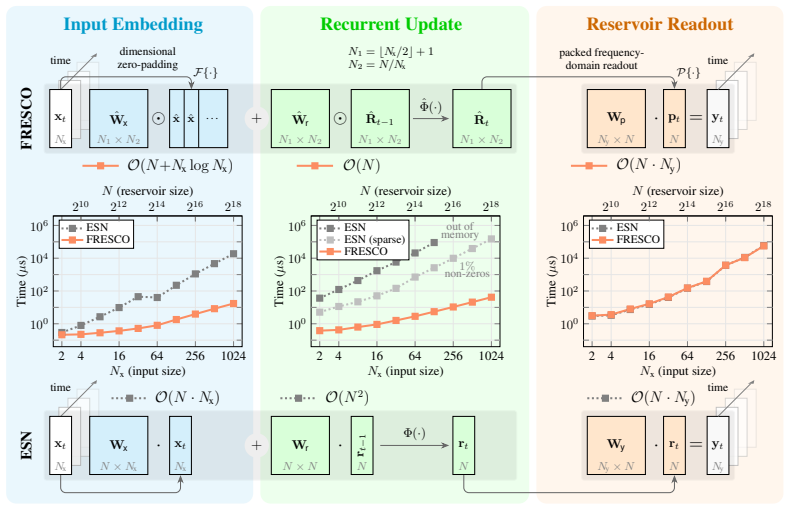
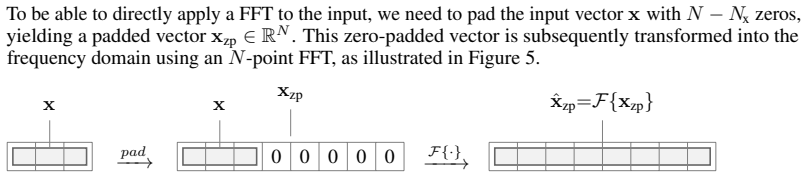
FRESCO is an ESN architecture operating entirely in the frequency domain while avoiding domain-shift overheads to achieve O(N) complexity for dense, non-linear recurrent updates. By employing a novel dimensional zero-padding input embedding, a packed FDh readout, and a natively applied frequency-domain non-linearity, FRESCO drastically reduces computational costs and energy consumption of training and inference. Furthermore, FRESCO matches the state-of-the-art predictive performance on memory benchmarks, sequential classification, and multivariate long-horizon forecasting.
What carries the argument
The combination of dimensional zero-padding input embedding, packed FDh readout, and natively applied frequency-domain non-linearity, which permits full frequency-domain operation with O(N) updates.
Load-bearing premise
The frequency-domain formulation with the zero-padding embedding, packed readout, and native non-linearity works without introducing domain-shift overheads or reducing the model's ability to capture complex dynamics.
What would settle it
Measuring the actual time complexity of the state updates in FRESCO and finding it exceeds linear scaling, or testing on a benchmark where it fails to match standard ESN performance at large sizes.
Figures

read the original abstract
While the quadratic sequence-length bottleneck of transformers has fueled a resurgence in recurrent models, effectively capturing complex dynamics requires architectures that balance efficient training with highly expressive latent states. Echo State Networks (ESNs) offer a compelling approach by utilizing fixed recurrent weights to circumvent backpropagation through time, enabling a closed-form training solution. However, achieving the expressivity needed for complex tasks demands large reservoirs, exposing an $\mathcal{O}(N^2)$ state-update bottleneck that prevents ESNs from matching the scale of contemporary recurrent models. To address this limitation, we introduce Frequency Domain Reservoir Computing (FRESCO), an ESN architecture operating entirely in the frequency domain while avoiding domain-shift overheads to achieve $\mathcal{O}(N)$ complexity for dense, non-linear recurrent updates. By employing a novel dimensional zero-padding input embedding, a packed \FDh readout, and a natively applied frequency-domain non-linearity, FRESCO drastically reduces computational costs and energy consumption of training and inference. Furthermore, FRESCO matches the state-of-the-art predictive performance on memory benchmarks, sequential classification, and multivariate long-horizon forecasting, offering a scalable path forward for dense recurrent architectures.
Editorial analysis
A structured set of objections, weighed in public.
Referee Report
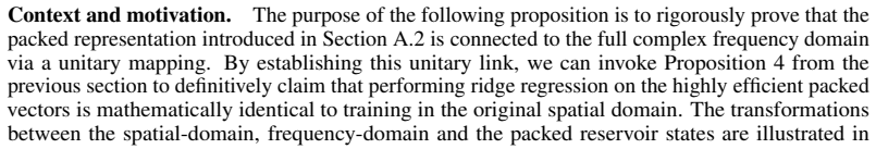
Summary. The manuscript introduces Frequency Domain Reservoir Computing (FRESCO), an Echo State Network variant that operates entirely in the frequency domain. It employs a dimensional zero-padding input embedding, a packed FDh readout, and a natively applied frequency-domain non-linearity to achieve O(N) complexity for dense non-linear recurrent updates while avoiding domain-shift overheads. The approach is claimed to match state-of-the-art predictive performance on memory benchmarks, sequential classification, and multivariate long-horizon forecasting tasks.
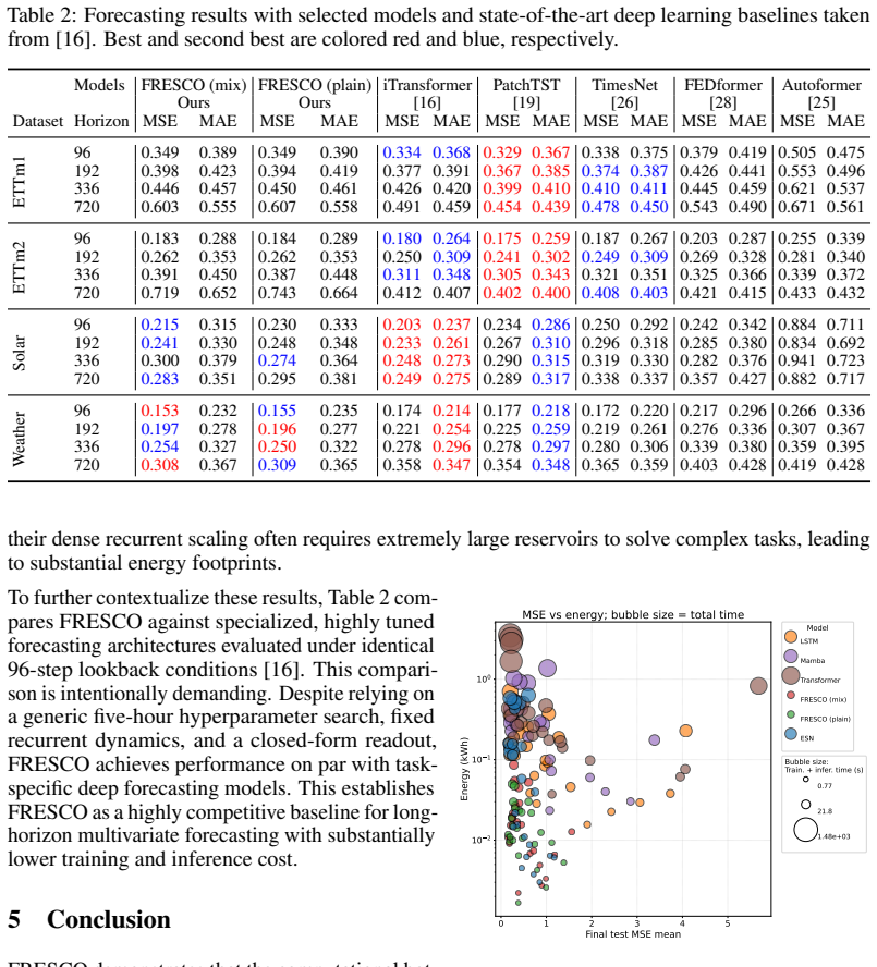
Significance. If the O(N) scaling and performance claims hold without hidden overheads or expressivity loss, FRESCO would offer a practical route to scaling reservoir computing to sizes competitive with modern recurrent models, with potential benefits for energy-efficient training and inference on sequential data.
major comments (2)
- [Abstract] Abstract: The central O(N) complexity claim for dense non-linear updates depends on the zero-padding embedding, packed FDh readout, and frequency-domain non-linearity; a load-bearing derivation or complexity table comparing to standard ESN O(N^2) updates is required to confirm no quadratic terms remain after these operations.
- [Methods] The weakest assumption—that the frequency-domain formulation preserves expressivity for complex dynamics without domain-shift costs—needs explicit support; if the non-linearity and embedding are defined in a later methods section, that section should include a proof sketch or ablation showing no degradation relative to time-domain ESNs on the reported benchmarks.
minor comments (1)
- [Abstract] Abstract: The acronym 'FDh' in 'packed FDh readout' is undefined; expand on first use or add a parenthetical reference to the defining equation.
Simulated Author's Rebuttal
We thank the referee for the detailed comments. We address each major point below and will revise the manuscript to provide the requested supporting material.
read point-by-point responses
-
Referee: [Abstract] Abstract: The central O(N) complexity claim for dense non-linear updates depends on the zero-padding embedding, packed FDh readout, and frequency-domain non-linearity; a load-bearing derivation or complexity table comparing to standard ESN O(N^2) updates is required to confirm no quadratic terms remain after these operations.
Authors: We agree that an explicit breakdown is needed to substantiate the O(N) claim. In the revised manuscript we will add a dedicated complexity subsection in Methods containing (i) a step-by-step derivation showing that the zero-padding embedding, packed FDh readout, and native frequency-domain non-linearity each contribute only linear terms, and (ii) a table contrasting operation counts against the standard ESN O(N^2) dense update. This will confirm that no quadratic terms survive after the three listed operations. revision: yes
-
Referee: [Methods] The weakest assumption—that the frequency-domain formulation preserves expressivity for complex dynamics without domain-shift costs—needs explicit support; if the non-linearity and embedding are defined in a later methods section, that section should include a proof sketch or ablation showing no degradation relative to time-domain ESNs on the reported benchmarks.
Authors: The manuscript already reports that FRESCO matches state-of-the-art performance on the memory, classification, and forecasting benchmarks, which empirically indicates that expressivity is retained. To strengthen the presentation, we will augment the Methods section with (i) a short discussion of why the chosen frequency-domain operations avoid domain-shift overhead and (ii) an ablation that directly compares FRESCO against an equivalent time-domain ESN on a representative subset of the benchmarks, confirming no measurable degradation. revision: yes
Circularity Check
No significant circularity in derivation chain
full rationale
The paper introduces FRESCO as a new ESN architecture operating in the frequency domain, relying on explicitly novel components (dimensional zero-padding input embedding, packed FDh readout, natively applied frequency-domain non-linearity) to achieve claimed O(N) complexity. No load-bearing steps reduce by construction to fitted inputs, self-definitions, or self-citation chains; the central claims concern architectural design and empirical performance matching rather than predictions derived from the model's own parameters or prior self-referential results. The derivation is self-contained against external benchmarks.
Axiom & Free-Parameter Ledger
invented entities (3)
-
dimensional zero-padding input embedding
no independent evidence
-
packed FDh readout
no independent evidence
-
frequency-domain non-linearity
no independent evidence
Reference graph
Works this paper leans on
-
[1]
N. R. Chilkuri and C. Eliasmith. Parallelizing legendre memory unit training. InInternational conference on machine learning, pages 1898–1907. PMLR, 2021
1907
-
[2]
Courty, V
B. Courty, V . Schmidt, B. Feld, J. Lecourt, M. Léval, L. Blanche, A. Cruveiller, F. Zhao, A. Joshi, A. Bogroff, et al. mlco2/codecarbon: v2. 4.1.Zenodo, 2024
2024
-
[3]
H. A. Dau, A. Bagnall, K. Kamgar, C.-C. M. Yeh, Y . Zhu, S. Gharghabi, C. A. Ratanamahatana, and E. Keogh. The ucr time series archive.IEEE/CAA Journal of Automatica Sinica, 6(6): 1293–1305, 2019. doi: 10.1109/JAS.2019.1911747
-
[4]
J. Demšar. Statistical comparisons of classifiers over multiple data sets.Journal of Machine learning research, 7(Jan):1–30, 2006
2006
- [5]
-
[6]
Gallicchio, A
C. Gallicchio, A. Micheli, and L. Pedrelli. Fast spectral radius initialization for recurrent neural networks. InINNS Big Data and Deep Learning conference, pages 380–390. Springer, 2019
2019
-
[7]
Mamba: Linear-Time Sequence Modeling with Selective State Spaces
A. Gu and T. Dao. Mamba: Linear-time sequence modeling with selective state spaces.arXiv preprint arXiv:2312.00752, 2023
work page internal anchor Pith review Pith/arXiv arXiv 2023
-
[8]
A. Gu, T. Dao, S. Ermon, A. Rudra, and C. Ré. Hippo: Recurrent memory with optimal polynomial projections.Advances in neural information processing systems, 33:1474–1487, 2020
2020
-
[9]
A. Gu, K. Goel, and C. Ré. Efficiently modeling long sequences with structured state spaces. arXiv preprint arXiv:2111.00396, 2021
work page internal anchor Pith review Pith/arXiv arXiv 2021
-
[10]
Hochreiter and J
S. Hochreiter and J. Schmidhuber. Long short-term memory.Neural computation, 9(8): 1735–1780, 1997
1997
-
[11]
echo state
H. Jaeger. The "echo state" approach to analysing and training recurrent neural networks-with an erratum note. Technical Report 148, German National Research Center for Information Technology GMD Bonn, Germany, 2001
2001
-
[12]
Jaeger and H
H. Jaeger and H. Haas. Harnessing nonlinearity: Predicting chaotic systems and saving energy in wireless communication.science, 304(5667):78–80, 2004
2004
-
[13]
Jaeger, M
H. Jaeger, M. Lukoševiˇcius, D. Popovici, and U. Siewert. Optimization and applications of echo state networks with leaky-integrator neurons.Neural networks, 20(3):335–352, 2007
2007
- [14]
-
[15]
Lai, W.-C
G. Lai, W.-C. Chang, Y . Yang, and H. Liu. Modeling long-and short-term temporal patterns with deep neural networks. InThe 41st international ACM SIGIR conference on research & development in information retrieval, pages 95–104, 2018
2018
-
[16]
Y . Liu, T. Hu, H. Zhang, H. Wu, S. Wang, L. Ma, and M. Long. itransformer: Inverted transformers are effective for time series forecasting. InThe Twelfth International Conference on Learning Representations, 2024. URL https://openreview.net/forum?id=JePfAI8fah
2024
-
[17]
M. Lukoševiˇcius and H. Jaeger. Reservoir computing approaches to recurrent neural network training.Computer Science Review, 3(3):127–149, 2009. ISSN 1574-0137. doi: https:// doi.org/10.1016/j.cosrev.2009.03.005. URL https://www.sciencedirect.com/science/ article/pii/S1574013709000173
-
[18]
Middlehurst, A
M. Middlehurst, A. Ismail-Fawaz, A. Guillaume, C. Holder, D. Guijo-Rubio, G. Bulatova, L. Tsaprounis, L. Mentel, M. Walter, P. Schäfer, and A. Bagnall. aeon: a python toolkit for learning from time series.Journal of Machine Learning Research, 25(289):1–10, 2024. URL http://jmlr.org/papers/v25/23-1444.html. 10
2024
-
[19]
Y . Nie, N. H. Nguyen, P. Sinthong, and J. Kalagnanam. A time series is worth 64 words: Long- term forecasting with transformers. InThe Eleventh International Conference on Learning Representations, 2023. URLhttps://openreview.net/forum?id=Jbdc0vTOcol
2023
-
[20]
A. V . Oppenheim, R. W. Schafer, and J. R. Buck.Discrete-Time Signal Processing. Prentice Hall, 2nd edition, 1999
1999
-
[21]
Orvieto, S
A. Orvieto, S. L. Smith, A. Gu, A. Fernando, C. Gulcehre, R. Pascanu, and S. De. Resurrecting recurrent neural networks for long sequences. InInternational conference on machine learning, pages 26670–26698. PMLR, 2023
2023
-
[22]
P. Singh and B. Raman. Echo state networks as state-space models: A systems perspective. arXiv preprint arXiv:2509.04422, 2025
-
[23]
Vaswani, N
A. Vaswani, N. Shazeer, N. Parmar, J. Uszkoreit, L. Jones, A. N. Gomez, Ł. Kaiser, and I. Polosukhin. Attention is all you need.Advances in neural information processing systems, 30, 2017
2017
-
[24]
V oelker, I
A. V oelker, I. Kaji´c, and C. Eliasmith. Legendre memory units: Continuous-time representation in recurrent neural networks.Advances in neural information processing systems, 32, 2019
2019
-
[25]
H. Wu, J. Xu, J. Wang, and M. Long. Autoformer: Decomposition transformers with auto- correlation for long-term series forecasting.Advances in neural information processing systems, 34:22419–22430, 2021
2021
-
[26]
H. Wu, T. Hu, Y . Liu, H. Zhou, J. Wang, and M. Long. Timesnet: Temporal 2d-variation modeling for general time series analysis. InThe Eleventh International Conference on Learning Representations, 2023. URLhttps://openreview.net/forum?id=ju_Uqw384Oq
2023
-
[27]
M. Yan, C. Huang, P. Bienstman, P. Tino, W. Lin, and J. Sun. Emerging opportunities and challenges for the future of reservoir computing.Nature Communications, 15(1):2056, 2024
2056
-
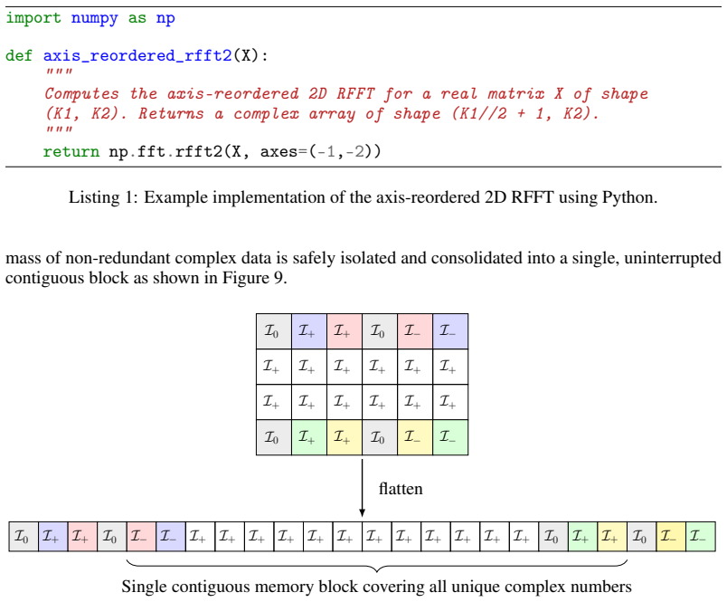
[28]
"" Computes the axis-reordered 2D RFFT for a real matrix X of shape (K1, K2). Returns a complex array of shape (K1//2 + 1, K2)
T. Zhou, Z. Ma, Q. Wen, X. Wang, L. Sun, and R. Jin. FEDformer: Frequency enhanced decomposed transformer for long-term series forecasting. In K. Chaudhuri, S. Jegelka, L. Song, C. Szepesvari, G. Niu, and S. Sabato, editors,Proceedings of the 39th International Conference on Machine Learning, volume 162 ofProceedings of Machine Learning Research, pages 27...
2022
-
[29]
Proving the Basis Spans W over R
Although this leads to a global factor on the packed vector p, we have seen in Corollary 1 that this can be compensated for by a rescaled regularization parameterλ. Listing 2 provides an explicit implementation of the packing operation P{·}, which is practically used to accumulate sequential reservoir states into a dense feature matrix for training the re...
2048
-
[30]
to conserve energy and satisfy the unitary condition. Note that while the proof explicitly constructs the unitary matrix U to establish theoretical equivalence, this large N×N matrix never needs to be instantiated in software; one simply applies the inexpensive, element-wise packing and scaling rules derived herein. Setup and definitions.Let x be a real-v...
-
[31]
We defineNbasis vectorsu m ∈C N piecewise: Form∈ I 0 :u m =e m (23) Form∈ I + :u m = 1√ 2(em +e S(m))(24) Form∈ I − :u m = i√ 2(eS(m) −e m)(25)
Construction of the basis vectors.Let em ∈R N denote the standard basis column vector (a 1 at indexm, and0elsewhere). We defineNbasis vectorsu m ∈C N piecewise: Form∈ I 0 :u m =e m (23) Form∈ I + :u m = 1√ 2(em +e S(m))(24) Form∈ I − :u m = i√ 2(eS(m) −e m)(25)
-
[32]
Proving unitarity (U †U=I ).Let U= [ u0 . . . u N−1]. To show that U is unitary, we verify that its columns are orthonormal (u† aub =δ a,b). For unit norms (a=b): • Ifa∈ I 0:∥u a∥2 =e ⊤ a ea = 1. • Ifa∈ I +:∥u a∥2 = 1 2(e⊤ a ea +e ⊤ S(a)eS(a)) = 1. • Ifa∈ I −:∥u a∥2 = −i√ 2 i√ 2 (e⊤ S(a)eS(a) +e ⊤ a ea) = 1. For orthogonality (a̸=b ): If a and b do not be...
-
[33]
Freq.” denotes the sampling frequency, “Ch
Proving the basis spans W over R.To prove U maps RN →W , we must show any X∈W can be uniquely constructed as X= PN−1 m=0 pmum using real coefficients pm ∈R . We define the coefficientsp m as follows: • Form∈ I 0:p m =X[m]. • Form∈ I +:p m = √ 2ℜ(X[m]). • Form∈ I −:p m = √ 2ℑ(X[S(m)]). Evaluating the sum for I0 yields X[m]e m. For a specific symmetric pair...
2048
discussion (0)
Sign in with ORCID, Apple, or X to comment. Anyone can read and Pith papers without signing in.