Painlev\'e \uppercase\expandafter{\romannumeral34\relax} and collisionless shock in the defocusing NLS equation with step-like initial data in the transition regions

Engui Fan; Yidan Zhang; Zhaoyu Wang

arxiv: 2606.26911 · v2 · pith:FD34PVRUnew · submitted 2026-06-25 · 🧮 math.AP · math-ph· math.MP

Painlev\'e uppercaseexpandafter{romannumeral34relax} and collisionless shock in the defocusing NLS equation with step-like initial data in the transition regions

Engui Fan , Zhaoyu Wang , Yidan Zhang This is my paper

Pith reviewed 2026-06-30 09:56 UTC · model grok-4.3

classification 🧮 math.AP math-phmath.MP

keywords defocusing NLSstep-like initial dataPainlevé XXXIVcollisionless shocknonlinear steepest descentRiemann-Hilbert problemlong-time asymptotics

0 comments

The pith

Long-time asymptotics for defocusing NLS with step-like data are given by Painlevé XXXIV formulas in two transition regions and Riemann theta functions in the collisionless shock region.

A machine-rendered reading of the paper's core claim, the machinery that carries it, and where it could break.

The paper derives the leading-order long-time asymptotic expansion of the solution to the Cauchy problem for the defocusing nonlinear Schrödinger equation with step-like initial data, specifically in three distinct transition regions. In the first two regions the expansion is expressed through Painlevé XXXIV-type formulas, while the third region is identified as a collisionless shock whose leading behavior is captured by Riemann theta functions. The derivation rests on applying the nonlinear steepest descent method to the Riemann-Hilbert formulation of the initial-value problem. A reader would care because these formulas supply explicit, computable descriptions of the solution precisely where standard soliton or dispersive asymptotics cease to apply.

Core claim

Using the nonlinear steepest descent method, the leading-order asymptotics in the first two transition regions are characterized by Painlevé XXXIV-type formula, while in the third collisionless shock region the leading-order asymptotics is described in terms of Riemann theta functions.

What carries the argument

The Riemann-Hilbert formulation of the Cauchy problem, to which the nonlinear steepest descent method is applied to obtain the asymptotics.

If this is right

The solution in the first two transition regions is governed at leading order by Painlevé XXXIV transcendentals.
The collisionless shock region exhibits oscillatory behavior captured by Riemann theta functions.
These expansions constitute the complete leading-order long-time description across the three identified transition zones.
The same Riemann-Hilbert setup and steepest-descent procedure yield explicit error estimates once the leading terms are subtracted.

Where Pith is reading between the lines

These are editorial extensions of the paper, not claims the author makes directly.

The same transition-region analysis may extend to other integrable equations whose Riemann-Hilbert problems admit analogous steepest-descent contours.
Physical observables such as intensity or momentum density in optical or fluid systems governed by defocusing NLS would inherit these Painlevé or theta-function signatures in the corresponding space-time windows.

Load-bearing premise

The Riemann-Hilbert formulation associated with the Cauchy problem admits the application of the nonlinear steepest descent method to derive the asymptotics in the transition regions.

What would settle it

Numerical integration of the defocusing NLS equation with the given step-like initial data that produces leading-order behavior in any of the three regions inconsistent with the stated Painlevé XXXIV or Riemann theta expressions.

Figures

Figures reproduced from arXiv: 2606.26911 by Engui Fan, Yidan Zhang, Zhaoyu Wang.

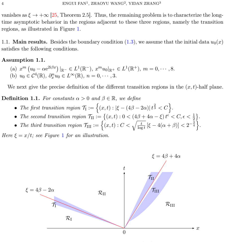
**Figure 1.** Figure 1: The different asymptotic regions of the (x, t)-half plane, where ξ = x/t Long-time asymptotics of the solution u(x, t) in each of the regions given in Definition 1.1 are main results of the present work. Theorem 1.2. Let u(x, t) be the global solution of the Cauchy problem (1.1)–(1.2) for the defocusing NLS equation over the real line under Assumption 1.1, and denote by r(k) the reflection coefficient. As… view at source ↗

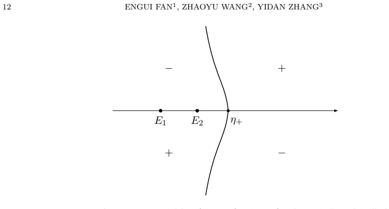
**Figure 2.** Figure 2: The signature table of Im gI for ξ ∈ TI , where “+” and “−” denote Im gI > 0 and Im gI < 0 in the corresponding regions, respectively. The solid line represents the level set where Img = 0, which asymptotes to the vertical line Rek = − ξ 4 . 3.1.1. RH problem for M(1) . By the function gI defined in (3.1), we introduce a new matrixvalued function M(1) by (3.4) M(1)(k) = M(1)(k; x, t) := e−itgI,∞(ξ)σ3M(k)e… view at source ↗

**Figure 3.** Figure 3: The jump contours Γ (3) and regions U (3) j , U(3)∗ j , j = 1, 2 of RH problem for M(3) when ξ ∈ TI . 3.3.2. RH problem for M(3) . Now we are ready to introduce a transformation (3.9) M(3)(k) = M(3)(k; x, t) := M(2)(k)D σ3 I (k)G(k)D −σ3 I (k), where (3.10) G(k) :=    [PITH_FULL_IMAGE:figures/full_fig_p015_3.png] view at source ↗

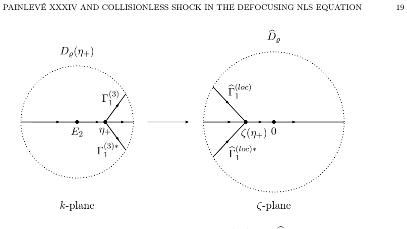
**Figure 4.** Figure 4: The map between Dϱ(η+) and Dbϱ. With respect to item (e) of Proposition 3.2, item (b) of Proposition 3.3 and the asymptotics of r(k) near E2 in Proposition 2.2, we have, for large t, DI(k) = e i 2 arg q2,0 + O(t −1/3+ϵ1/2 ), |ra(k) − r(E2)| ≲ |k − E2| 1/2 + |k − E2|e t 4 |ImgI| ≲ t −1/3+ϵ1/2 + t −2/3+ϵ1 e t 4 |ImgI| , k ∈ Dϱ(E2) ∩ C +. which implies that for k ∈ Dϱ(E2) ∩ C +, |D −2 I (k)ra(k) − D −2 I (E2)… view at source ↗

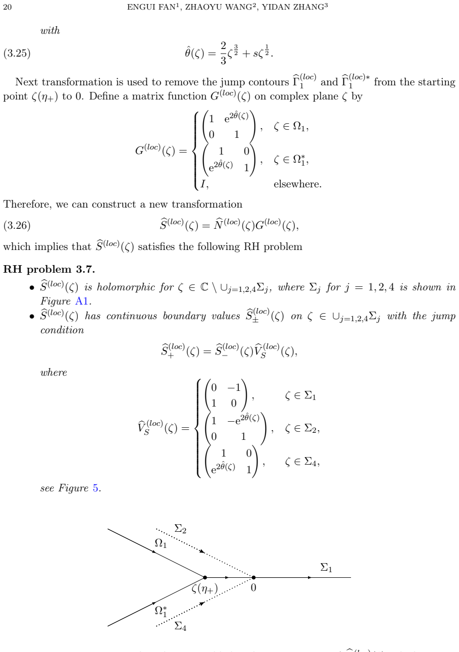
**Figure 5.** Figure 5: Two auxiliary lines are added to the jump contour of Nb(loc) (ζ), which can be deformed into the Painlevé XXXIV model [PITH_FULL_IMAGE:figures/full_fig_p020_5.png] view at source ↗

**Figure 6.** Figure 6: The jump contours Γ (err) of RH problem for M(err) for ξ ∈ TI . Using item (c) in Proposition 3.3, item (c) in Proposition 3.4, Proposition 3.6 and Lemma 3.7, a straightforward calculation yields the following proposition. Proposition 3.8. For ξ ∈ TI , the function V (err) (·) − I : Γ(err) → C 2×2 lies in L p [PITH_FULL_IMAGE:figures/full_fig_p025_6.png] view at source ↗

**Figure 7.** Figure 7: The signature table of Im gII for ξ ∈ TII, where “+” and “−” denote Im gII > 0 and Im gII < 0 in the corresponding regions, respectively [PITH_FULL_IMAGE:figures/full_fig_p028_7.png] view at source ↗

**Figure 8.** Figure 8: The jump contours Γ (3) and regions U (3) j , U(3)∗ j , j = 1, 2 of RH problem for M(3) when ξ ∈ TII. Now we are ready to introduce a transformation (4.9) M(3)(k) = M(3)(k; x, t) := M(2)(k)D σ3 II (k)G(k)D −σ3 II (k), where (4.10) G(k) :=    [PITH_FULL_IMAGE:figures/full_fig_p031_8.png] view at source ↗

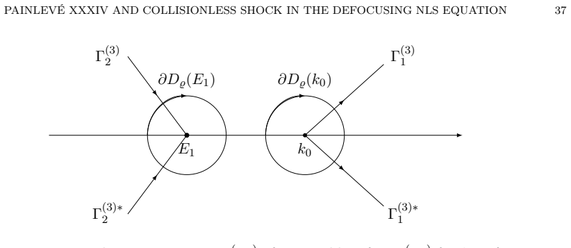
**Figure 9.** Figure 9: The jump contours Γ (loc,y) of RH problem for M(loc,y) for y ∈ {E1, k0} when ξ ∈ TII. As to the local parametrix near E1, it can be also be constructed by the Painlevé XXXIV parametrix shown in Appendix A in a standard manner. We recall the asymptotics of gII near E1 that gII(k) = −2(k0 − E1) 3 2 (E1 − k) 1 2 − 3(k0 − E1) 1 2 (E1 − k) 3 2 + O((E1 − k) 5 2 ) [PITH_FULL_IMAGE:figures/full_fig_p033_9.png] view at source ↗

**Figure 10.** Figure 10: The jump contours Γ (err) of RH problem for M(err) for ξ ∈ TII. Using Lemma 4.4 and Lemma 4.5, a straightforward calculation yields the following proposition. Proposition 4.6. For ξ ∈ TII, the function V (err) (·) − I : Γ(err) → C 2×2 lies in L p [PITH_FULL_IMAGE:figures/full_fig_p037_10.png] view at source ↗

**Figure 11.** Figure 11: The signature table of Im θ(k) for ξ ∈ TIII, where “+” and “−” denote Im gI > 0 and Im gI < 0 in the corresponding regions, respectively. 5.1. First transformation: M → M(1) . In this section, we rewrite the phase factor e itθ(k) into a simpler way which relocates the saddle point k0 to −1 and E1 to 0 respectively. Introduce the following changes of variables (5.1) z = k − E1 E1 − k0 , τ = t[ξ − 4(α + β)]… view at source ↗

**Figure 12.** Figure 12: The homology basis of the Riemann surface M associated with w(z) = p (z 2 − a 2)(z 2 − b 2). The a1-cycle is closed counterclockwise oriented simple loop around the cut [a, b] and the b1-cycle starts on the upper sheet of the cut [a, b], goes to the cut [−b, −a], proceeds to the lower sheet, and then returns to the starting point. Therefore, the g-function for ξ ∈ TIII is defined by (5.5) gIII(z) = gIII(z… view at source ↗

**Figure 13.** Figure 13: The signature table of Im gIII for ξ ∈ TIII, where “+” and “−” denote Im gIII > 0 and Im gIII < 0 in the corresponding regions, respectively. By the signature table of Im gIII in [PITH_FULL_IMAGE:figures/full_fig_p041_13.png] view at source ↗

**Figure 14.** Figure 14: The jump contours Γ (4) and regions U (4) j , U(4)∗ j , j = 1, 2, 3 of RH problem for M(4) when ξ ∈ TIII. Now we are ready to define matrix-valued function M(4) by (5.16) M(4)(z) = M(4)(z; x, t) := M(3)(k)δ σ3 (z)G(z)δ(z) −σ3 , [PITH_FULL_IMAGE:figures/full_fig_p043_14.png] view at source ↗

read the original abstract

We consider the Cauchy problem for the defocusing nonlinear Schr\"odinger (NLS) equation with step-like initial data. Using the nonlinear steepest descent method, we derive the long-time asymptotic expansion of the solution to the Cauchy problem in three distinct transition regions. In the first two transition regions, the leading-order asymptotics are characterized by Painlev\'e \uppercase\expandafter{\romannumeral34\relax}-type formula, while in the third one is a collisionless shock region, the leading-order asymptotics is describedin terms of Riemann theta functions. Our analysis is based on the Riemann-Hilbert formulation associated with the Cauchy problem of the defocusing NLS equation.

Editorial analysis

A structured set of objections, weighed in public.

Desk editor's note, referee report, simulated authors' rebuttal, and a circularity audit. Tearing a paper down is the easy half of reading it; the pith above is the substance, this is the friction.

Desk Editor's Note private letter to a colleague

Abstract claims Painlevé XXXIV asymptotics in two transition regions and Riemann theta in a collisionless shock for defocusing NLS step-like data, but nothing can be checked without the full text.

read the letter

The abstract says the authors use nonlinear steepest descent on the Riemann-Hilbert problem for defocusing NLS with step-like initial data to get leading asymptotics in three transition regions: Painlevé XXXIV type in the first two, and Riemann theta functions in the third, which they call a collisionless shock region.

That is the stated contribution. It takes the standard RH setup for this initial-value problem and applies the method to these particular zones between the different long-time regimes.

The abstract is clear about which special functions appear where. That part is straightforward to state.

The problem is that only the abstract exists here. No contour pictures, no g-function, no error bounds, no matching arguments. The stress-test note is correct: the central claims sit on steps that cannot be inspected. We therefore cannot tell whether the derivations hold, whether the regions are defined sharply enough, or whether this overlaps with earlier results on similar step-like problems.

This is aimed at people already working on long-time asymptotics for integrable equations, especially those who follow the Deift-Zhou steepest-descent machinery for NLS. A specialist in that corner would want to see the full paper to decide if the claims add something usable.

It is worth sending the full version to a referee if the technical details are there. The topic is narrow but fits the subfield, and the claims are specific enough that a proper review makes sense once the text is available.

Referee Report

1 major / 1 minor

Summary. The manuscript considers the Cauchy problem for the defocusing nonlinear Schrödinger equation with step-like initial data. Using the Riemann-Hilbert formulation and the nonlinear steepest descent method, it derives the long-time asymptotic expansion in three transition regions, claiming Painlevé XXXIV-type leading-order asymptotics in the first two regions and a description in terms of Riemann theta functions in the third collisionless shock region.

Significance. If the technical steps are valid, the results would extend the asymptotic analysis of integrable PDEs to transition zones with step-like data, providing explicit special-function characterizations that connect different regimes; this is of interest in the mathematical theory of nonlinear dispersive equations.

major comments (1)

Abstract: the central claim that the RH problem admits nonlinear steepest descent yielding the stated Painlevé XXXIV and theta-function characterizations rests on unprovided technical elements (contour deformations, g-function, error estimates, and matching arguments). Without these, the applicability in the transition regions cannot be assessed and the claims remain unverifiable from the manuscript text.

minor comments (1)

Abstract: 'describedin' is missing a space and should read 'described in'.

Simulated Author's Rebuttal

1 responses · 0 unresolved

We thank the referee for their report. We address the single major comment below.

read point-by-point responses

Referee: [—] Abstract: the central claim that the RH problem admits nonlinear steepest descent yielding the stated Painlevé XXXIV and theta-function characterizations rests on unprovided technical elements (contour deformations, g-function, error estimates, and matching arguments). Without these, the applicability in the transition regions cannot be assessed and the claims remain unverifiable from the manuscript text.

Authors: The manuscript contains the Riemann-Hilbert formulation for the Cauchy problem and carries out the nonlinear steepest descent analysis, including the required contour deformations, g-function construction, error estimates, and matching arguments, in the sections following the abstract. These steps justify the Painlevé XXXIV leading-order terms in the first two transition regions and the Riemann theta-function description in the collisionless shock region. The abstract is a summary only; the technical details appear in the body of the paper. revision: no

Circularity Check

0 steps flagged

No circularity; derivation applies established RH steepest-descent framework to new initial data

full rationale

The abstract states that the long-time asymptotics are derived via the nonlinear steepest descent method applied to the Riemann-Hilbert formulation of the defocusing NLS Cauchy problem with step-like data, yielding Painlevé XXXIV in the first two transition regions and Riemann theta functions in the collisionless shock region. No self-definitional equations, fitted parameters renamed as predictions, load-bearing self-citations, uniqueness theorems imported from the authors' prior work, or ansatzes smuggled via citation appear in the text. The claimed results rest on external, independently verifiable analytic machinery rather than reducing to the paper's own inputs by construction.

Axiom & Free-Parameter Ledger

0 free parameters · 1 axioms · 0 invented entities

Abstract-only review provides no explicit free parameters, invented entities, or detailed axioms beyond the stated reliance on the Riemann-Hilbert formulation.

axioms (1)

domain assumption The Cauchy problem for the defocusing NLS equation with step-like initial data admits a Riemann-Hilbert formulation.
Invoked in the abstract as the basis for the nonlinear steepest descent analysis.

pith-pipeline@v0.9.1-grok · 5639 in / 1162 out tokens · 31834 ms · 2026-06-30T09:56:37.541065+00:00 · methodology

Review history (2 revisions) →