Dissipative phase decision without ground-state preparation
Pith reviewed 2026-06-30 09:53 UTC · model grok-4.3
The pith
Dissipative evolution under tailored jump operators reveals the ground-state phase from low-energy observables at early times without accurate ground-state preparation.
A machine-rendered reading of the paper's core claim, the machinery that carries it, and where it could break.
Core claim
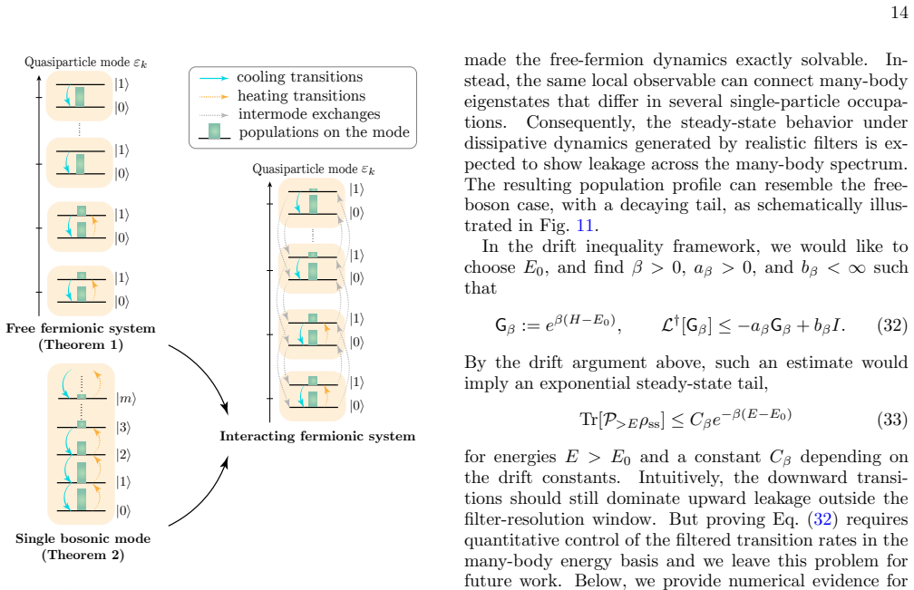
Rather than determining the phase by preparing highly accurate approximations to ground states, we prepare a representative state of a candidate phase and monitor the early-time response of phase-sensitive observables under cooling dynamics tailored to the target Hamiltonian. For a class of phase-decision problems in which the relevant observables can be inferred from the low-energy manifold, and with jump operators implementable using only short-time Hamiltonian simulation, the dissipative evolution rapidly suppresses high-energy components and drives the system into a low-energy manifold whose observables already reveal the underlying ground-state phase, well before mixing to the steady st
What carries the argument
Tailored dissipative cooling dynamics whose jump operators are realized by short-time Hamiltonian simulation; the dynamics suppress high-energy components to access a low-energy manifold whose observables encode the ground-state phase.
If this is right
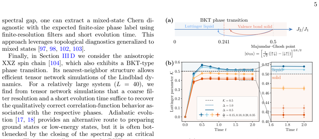
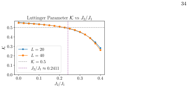
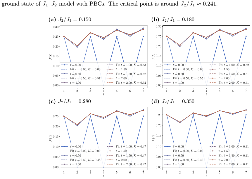
- Coarse filter resolutions and short evolution times suffice to recover phase-sensitive quantities such as the Luttinger parameter and topological diagnostics.
- The strategy applies to the frustrated J1-J2 Heisenberg chain, the Kitaev honeycomb model, and the XXZ chain, including Berezinskii-Kosterlitz-Thouless and topological phase transitions.
- Cooling dynamics with the described jump operators can rigorously prepare low-energy manifolds for free-fermionic and free-bosonic systems.
- Phase decision becomes a plausible target for future utility-scale studies on early fault-tolerant quantum devices.
Where Pith is reading between the lines
- The method may reduce circuit depth requirements for phase identification on near-term quantum hardware by replacing deep ground-state preparation circuits with shorter dissipative evolution.
- The same low-energy-manifold principle could be tested in other open-system protocols where only partial thermalization is feasible.
- Optimal design of jump operators for strongly interacting cases remains open and could be explored by varying the short-time Hamiltonian segments used to implement them.
Load-bearing premise
The assumption that phase-sensitive observables can be inferred from the low-energy manifold reached by the tailored dissipative dynamics.
What would settle it
A numerical simulation of one of the demonstrated models in which the early-time phase-sensitive observables after the proposed cooling fail to match the known ground-state phase indicators.
Figures


read the original abstract
We propose a dynamical approach to identifying ground-state quantum phases through short-time dissipative cooling. Rather than determining the phase by preparing highly accurate approximations to ground states, we prepare a representative state of a candidate phase and monitor the early-time response of phase-sensitive observables under cooling dynamics tailored to the target Hamiltonian. For a class of phase-decision problems in which the relevant observables can be inferred from the low-energy manifold, and with jump operators implementable using only short-time Hamiltonian simulation, the dissipative evolution rapidly suppresses high-energy components and drives the system into a low-energy manifold whose observables already reveal the underlying ground-state phase, well before mixing to the steady state. We demonstrate this strategy for the frustrated $J_1$--$J_2$ Heisenberg chain, the Kitaev honeycomb model, and the XXZ chain, including Berezinskii--Kosterlitz--Thouless and topological phase transitions. In particular, coarse filter resolutions and short evolution times suffice to recover phase-sensitive quantities such as the Luttinger parameter and topological diagnostics. We further provide theoretical justification that cooling dynamics with such jump operators can rigorously prepare low-energy manifolds for free-fermionic and free-bosonic systems, and investigate this mechanism for interacting fermionic systems. Our results suggest that phase decision is a plausible target for future utility-scale studies on early fault-tolerant quantum devices.
Editorial analysis
A structured set of objections, weighed in public.
Referee Report
Summary. The manuscript proposes a dynamical approach to ground-state phase decision via short-time dissipative cooling. Rather than preparing accurate ground states, tailored jump operators (implementable via short-time Hamiltonian simulation) drive the system into a low-energy manifold whose phase-sensitive observables reveal the underlying phase well before steady-state mixing. The strategy is demonstrated numerically on the frustrated J1-J2 Heisenberg chain, Kitaev honeycomb model, and XXZ chain (including BKT and topological transitions), with rigorous justification that the dynamics prepare low-energy manifolds for free-fermionic and free-bosonic systems and numerical investigation of the mechanism for interacting fermionic systems.
Significance. If the early-time manifold suppression holds, the approach could enable phase identification on early fault-tolerant devices with substantially reduced evolution times and without full ground-state preparation. The paper's explicit distinction between rigorous free-system guarantees and numerical interacting demonstrations is a strength, as is the coverage of multiple models and diagnostics such as the Luttinger parameter. The result is of interest for near-term quantum simulation but its broader impact depends on establishing greater generality beyond the specific numerics shown.
major comments (2)
- [Abstract] Abstract: the central claim is framed for a class of phase-decision problems that includes interacting models (frustrated J1-J2 Heisenberg chain, XXZ chain), yet the manuscript supplies rigorous preparation guarantees only for free-fermionic and free-bosonic systems while relying on model-specific numerical investigation for interacting cases. This distinction is load-bearing for the stated applicability.
- [Theoretical justification] Theoretical justification paragraph: the statement that the mechanism is investigated for interacting fermionic systems does not include a general proof that the low-energy manifold reached by the dissipative dynamics encodes the ground-state phase for arbitrary interacting Hamiltonians; the demonstrations remain specific to the three models studied.
Simulated Author's Rebuttal
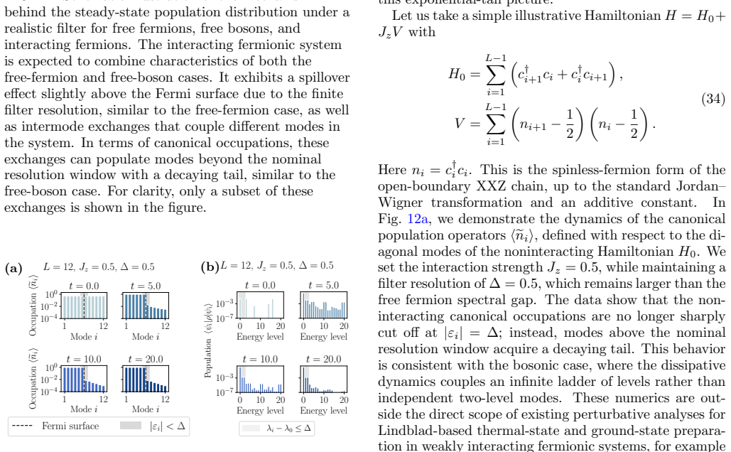
We thank the referee for their careful reading of the manuscript and for highlighting the importance of clearly delineating the scope of our rigorous results from our numerical demonstrations. We address each major comment below and will make the requested clarifications in a revised version.
read point-by-point responses
-
Referee: [Abstract] Abstract: the central claim is framed for a class of phase-decision problems that includes interacting models (frustrated J1-J2 Heisenberg chain, XXZ chain), yet the manuscript supplies rigorous preparation guarantees only for free-fermionic and free-bosonic systems while relying on model-specific numerical investigation for interacting cases. This distinction is load-bearing for the stated applicability.
Authors: We agree that the abstract should more explicitly distinguish the rigorous guarantees (limited to free-fermionic and free-bosonic systems) from the numerical evidence for interacting models. We will revise the abstract to state that the strategy is demonstrated numerically for the J1-J2 Heisenberg chain, Kitaev honeycomb model, and XXZ chain, while rigorous low-energy manifold preparation is proven only for free systems. revision: yes
-
Referee: [Theoretical justification] Theoretical justification paragraph: the statement that the mechanism is investigated for interacting fermionic systems does not include a general proof that the low-energy manifold reached by the dissipative dynamics encodes the ground-state phase for arbitrary interacting Hamiltonians; the demonstrations remain specific to the three models studied.
Authors: We acknowledge that the manuscript provides no general proof for arbitrary interacting Hamiltonians and that the demonstrations are specific to the three models. We will revise the theoretical justification paragraph to emphasize that the mechanism is investigated numerically for these specific cases and that a general proof for all interacting systems lies outside the present scope. revision: yes
Circularity Check
No significant circularity; derivation self-contained
full rationale
The paper introduces a dissipative cooling strategy for phase identification, with explicit separation between rigorous guarantees (free-fermion/boson systems) and numerical investigation (interacting models like J1-J2 and XXZ). No equations, fitted parameters, or self-citations are shown to reduce any central claim to a tautology or input by construction. The low-energy manifold inference and jump-operator implementation are presented as independent assumptions whose validity is tested externally via simulation and free-system proofs, not derived from the target observables themselves. This matches the default expectation of non-circularity for a methods paper whose core content is a new dynamical protocol rather than a closed algebraic reduction.
Axiom & Free-Parameter Ledger
Reference graph
Works this paper leans on
-
[1]
The term “bulk” means that we apply the coupling on all sites of the system
Free fermionic systems Let us consider a general quadratic fermionic Hamiltonian H= LX i,j=1 Fijc† i cj,(B7) and bulk coupling operators{c † i , ci}L i=1 to construct the Lindbladian jump operators for dissipative cooling dynamics. The term “bulk” means that we apply the coupling on all sites of the system. We first simplify the free-fermionic Hamiltonian...
-
[2]
Diagonalize the Hermitian matrixF=Udiag(ε k)L k=1U †, and chooseec† k =PL j=1 Ujk c† j such that H= LX k=1 εkec† keck.(B8) We calleck the canonical modes and assumeε k ̸= 0 for allk
-
[3]
Here we usen k to denote the quasiparticle number operator on thek-th canonical mode, i.e
Apply the particle–hole transformation bk := ( eck,ifε k >0, ec† k,ifε k <0, (B9) so that each mode has positive excitation energyλ k: H=E 0 + LX k=1 |εk|b† kbk =:E 0 + LX k=1 λkb† kbk =E 0 + LX k=1 λknk,(B10) A ground state is the quasiparticle vacuum state|ψ 0⟩=|0⟩ b satisfyingb k |ψ0⟩= 0 for allk, and the ground state energy isE 0 = P k:εk<0 εk. Here w...
-
[4]
The Hamiltonian and the coupling operator are H= Ωa †a=: ΩN(Ω>0), A=a+a †.(B35) Here N:=a †a(B36) is the number operator
Free bosonic systems We begin with the single bosonic mode. The Hamiltonian and the coupling operator are H= Ωa †a=: ΩN(Ω>0), A=a+a †.(B35) Here N:=a †a(B36) is the number operator. Using free-bosonic version of the Thouless theorem Eq. (B17), we have eiHs ae−iHs =e −iΩsa, e iHs a†e−iHs =e iΩsa†.(B37) Therefore, the jump operator is constructed as K= Z ∞ ...
-
[5]
squeezed number operator
Additional results on free bosonic systems Since the steady state is a Gaussian state, we could also understand the free bosonic systems by directly solving the steady state or the covariance matrix. In this section, we present some additional results about the steady state of the free bosonic system such as the trace-distance convergence and the generali...
-
[6]
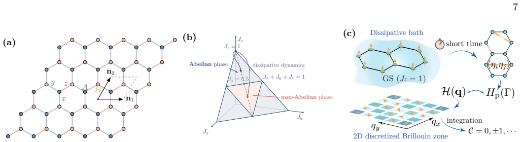
Kitaev honeycomb model Besides the Chern number, another phase-sensitive diagnostic for this phase transition is the mutual information between the two sites in the unit cell [153], which can be computed as I(sA,sB) = 1−H b 1 2 + 2⟨Sz sASz sB⟩ ,(D2) since for the states considered here the reduced density matrix of the two sites has an explicit form ρsA,s...
-
[7]
The results are shown in Fig
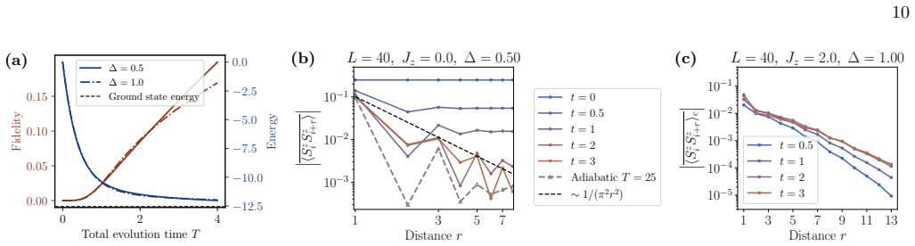
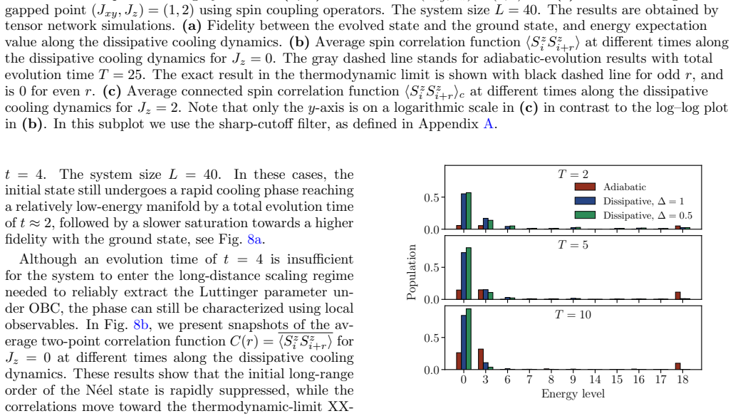
Trends in the realistic cooling dynamics for free and interacting systems Free fermions.We provide more results on the dissipative cooling for the tight-binding model that is equivalent to the XX model by Jordan–Wigner transformation H= L−1X i=1 (c† i+1ci +c † i ci+1).(D4) Here we apply the same setting of the initial state and jump operators as in Sectio...
2010
-
[8]
The gauge field is defined on the bonds as uij := 2iηα i ηα j (E2) ifi, jare connected by anα-type bond. It is easy to check that for any bonds⟨i, j⟩ α(i,j) and⟨k, l⟩ α(k,l), the gauge field satisfies the constraint [uij,u kl] = 0,[u ij, H] = 0.(E3) This means that each operatoru ij, together with the Hamiltonian can be simultaneously diagonalized in some...
-
[9]
We will discuss the details of the simulation of the dissipative dynamics in Section G 2
Chern number and purity gap We could probe the topological properties of the states along the dissipative dynamics by evaluating the Chern number of the covariance matrix Γ in the real space, defined as Γsµ,tν = i 2 Tr (ρ[ηsµ, ηtν]) = i⟨ηsµηtν⟩ − i 2 δsµ,tν, µ, ν=A, B,(F1) which only involves the two-point correlation functions in the real space and can b...
-
[10]
A simple mechanism for dissipative preparation of Chern insulators We explain how dissipative protocols can evade the unitary topological obstruction to preparing a Chern insulator. Consider a general two-band Chern insulator with Bloch Hamiltonian [155] H(q) =d(q)·σ= dz(q)d x(q)−id y(q) dx(q) + idy(q)−d z(q) ,σ= (σ x, σy, σz),(F13) The Qi–Wu–Zhang model ...
-
[11]
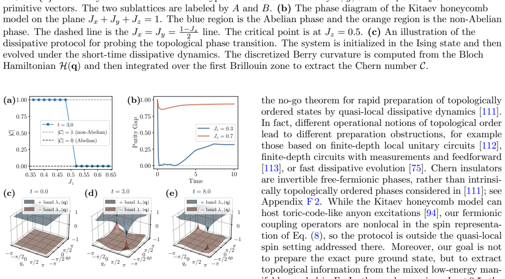
Probing the topological properties with realistic filters In Section III C, we demonstrate that the ground-state topological phase of the Kitaev honeycomb model can be probed by computing the Chern number directly from finite-filter-resolution dissipative dynamics. Following the approach in [97], computing the Chern number only requires distinguishing the...
-
[12]
pure N´ eel state
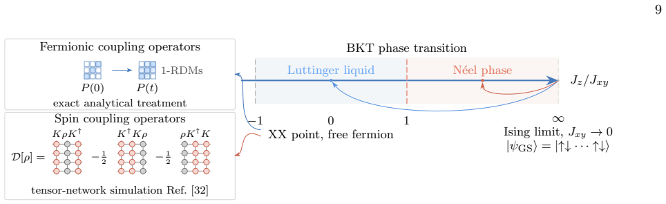
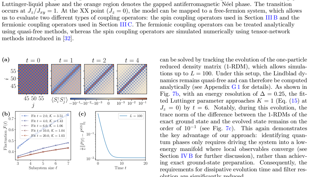
The XX model with bulk cooling a. Solving the 1-RDM dynamics We recall that the XX model can be fermionized into a free fermionic model by the Jordan–Wigner transformation, and the resulting Hamiltonian is given by Eq. (26). We consider the bulk cooling, where the coupling operators are chosen as the local fermionic creation and annihilation operators{c i...
-
[13]
anomalous
The Kitaev honeycomb model with local Majorana cooling a. Solving the covariance matrix dynamics We next discuss the Kitaev honeycomb model, where the jump operators are chosen as the local Majorana operators {ηsA, ηsB}s. We recall that, after fixing theZ 2 gauge and diagonalizing the Hamiltonian as discussed in Appendix E, the Kitaev honeycomb model can ...
discussion (0)
Sign in with ORCID, Apple, or X to comment. Anyone can read and Pith papers without signing in.