Estimating Free Energy Differences with Virtually Escorted Trajectories
Pith reviewed 2026-06-30 03:51 UTC · model grok-4.3
The pith
A virtual control field generates infinitely many work-like quantities from the same trajectories, each satisfying the fluctuation theorem for free energy differences.
A machine-rendered reading of the paper's core claim, the machinery that carries it, and where it could break.
Core claim
For a system driven irreversibly from equilibrium state A to B, the free energy difference ΔF can be estimated using the work fluctuation theorem. Adding a virtual control field u_θ that does not modify the underlying dynamics allows construction of work-like quantities W_θ such that the average of exp(-W_θ/T) equals exp(-ΔF/T) for any choice of θ. The parameters θ are selected to optimize convergence of the estimate from a given collection of trajectories, and conditions are identified under which the estimator has zero variance.
What carries the argument
The virtual control field u_θ, which redefines work without changing the physical trajectories, to produce an infinite family of equivalent fluctuation-theorem estimators.
If this is right
- The same set of trajectories can be reused to obtain improved free energy estimates by selecting an optimal θ after the fact.
- Variance reduction is achieved without generating additional trajectories or altering the simulation protocol.
- Under conditions where the virtual field makes W_θ independent of the random work fluctuations, the estimator variance reaches zero.
- The approach borrows from escorted estimation but applies the escorting only virtually to the work definition.
Where Pith is reading between the lines
- The method could lower the number of trajectories needed in molecular dynamics calculations of binding affinities.
- Similar virtual adjustments might be applied to other nonequilibrium theorems such as those for entropy production.
- The zero-variance condition provides a concrete test case in exactly solvable models like driven harmonic oscillators.
- Links to diffusion models suggest the parameter optimization step could be automated with machine-learning techniques.
Load-bearing premise
The virtual control field does not modify the underlying dynamics of the system.
What would settle it
A simulation in which the average of exp(-W_θ/T) over trajectories deviates from exp(-ΔF/T) for some choice of θ would falsify the claim that all such W_θ obey the fluctuation theorem.
Figures

read the original abstract
For a process in which a system is driven irreversibly from equilibrium state $A$ toward equilibrium state $B$, the free energy difference $\Delta F = F_B-F_A$ can be estimated using the work fluctuation theorem $\langle e^{-W/T}\rangle = e^{-\Delta F/T}$, where $W$ and $T$ denote work and temperature. The estimate often suffers from poor convergence with the number of trajectories used to calculate the average. Borrowing ideas from escorted free energy estimation, and from diffusion models of machine learning, we show how to construct infinitely many work-like quantities, $W_\theta$, that satisfy $\langle e^{-W_\theta/T}\rangle = e^{-\Delta F/T}$, for the same underlying dynamics. Our method involves a virtual control field ${\boldsymbol u}_\theta$ that does not modify these dynamics. We show how to choose parameter values $\theta$ to optimize convergence of the free energy estimate, for a fixed set of trajectories. We identify conditions under which our method provides a zero-variance estimator of $\Delta F$. We use numerical simulations of model systems to illustrate the gains in convergence that our method can achieve.
Editorial analysis
A structured set of objections, weighed in public.
Referee Report
Summary. The paper claims to construct infinitely many work-like quantities W_θ using a virtual control field u_θ that does not modify the underlying dynamics, such that ⟨e^{-W_θ/T}⟩ = e^{-ΔF/T} holds exactly on the original trajectory measure. It describes optimization of θ for improved convergence of the free energy estimate from a fixed set of trajectories and identifies conditions for zero-variance estimators, illustrated via numerical simulations on model systems.
Significance. If the construction is valid without hidden dynamical assumptions, the approach would allow post hoc optimization over a family of fluctuation-theorem estimators, potentially reducing the number of trajectories needed for accurate ΔF estimates in nonequilibrium simulations. The zero-variance conditions, if explicitly achievable, represent a notable theoretical strength.
major comments (2)
- [Derivation of fluctuation theorem for W_θ (likely §2–3)] The validity of ⟨e^{-W_θ/T}⟩ = e^{-ΔF/T} for virtual W_θ requires an exact path-measure cancellation (via Girsanov or equivalent Radon–Nikodym factor) that is absorbed into the definition of W_θ. The manuscript must provide the explicit derivation, including the assumed SDE form (e.g., overdamped Langevin with additive noise) and any divergence or continuity-equation conditions on u_θ, because this is load-bearing for the central claim that the equality holds for arbitrary u_θ on unmodified trajectories.
- [Optimization of θ and zero-variance conditions] The optimization procedure for θ and the explicit functional form of u_θ must be stated with sufficient detail to verify that the resulting estimator remains unbiased and that the zero-variance conditions are attainable without circularity or additional sampling; the abstract provides no equations for these steps.
minor comments (2)
- [Introduction] Clarify the precise relationship to prior escorted free-energy methods and diffusion-model literature with one or two additional citations in the introduction.
- Ensure all notation for W_θ, u_θ, and the parameter set θ is defined before first use in the main text.
Simulated Author's Rebuttal
We thank the referee for their careful review and constructive suggestions. We address each major comment below and will incorporate clarifications into a revised manuscript.
read point-by-point responses
-
Referee: [Derivation of fluctuation theorem for W_θ (likely §2–3)] The validity of ⟨e^{-W_θ/T}⟩ = e^{-ΔF/T} for virtual W_θ requires an exact path-measure cancellation (via Girsanov or equivalent Radon–Nikodym factor) that is absorbed into the definition of W_θ. The manuscript must provide the explicit derivation, including the assumed SDE form (e.g., overdamped Langevin with additive noise) and any divergence or continuity-equation conditions on u_θ, because this is load-bearing for the central claim that the equality holds for arbitrary u_θ on unmodified trajectories.
Authors: We agree that the derivation requires greater explicitness. The manuscript assumes the standard overdamped Langevin dynamics with additive white noise and derives the fluctuation theorem for W_θ via the Girsanov change-of-measure factor absorbed into the definition of the virtual work. In the revision we will add a self-contained derivation in §2 that starts from the SDE, states the precise form of the Radon–Nikodym derivative, and lists the required regularity conditions (divergence of u_θ and continuity-equation compatibility) under which the equality holds exactly for any sufficiently regular u_θ on the original trajectory measure. revision: yes
-
Referee: [Optimization of θ and zero-variance conditions] The optimization procedure for θ and the explicit functional form of u_θ must be stated with sufficient detail to verify that the resulting estimator remains unbiased and that the zero-variance conditions are attainable without circularity or additional sampling; the abstract provides no equations for these steps.
Authors: We will expand §3 and the methods section to give the explicit parametric form of u_θ(θ) and the post-hoc optimization criterion (minimization of the sample variance of e^{-W_θ/T} subject to the fixed trajectory ensemble). Because the fluctuation-theorem identity holds for every admissible θ, the estimator remains unbiased for any choice; the optimization merely selects the θ that yields the lowest variance on the given data. The zero-variance conditions are derived analytically as the existence of a u_θ that makes W_θ = ΔF almost surely; they do not require extra sampling and will be stated with the corresponding functional equation in the revision. revision: yes
Circularity Check
No circularity: virtual W_θ construction extends fluctuation theorem via independent path-measure adjustment
full rationale
The derivation introduces a virtual control field u_θ that leaves the underlying stochastic trajectories unchanged while redefining the work functional W_θ so that the exponential average remains exactly e^{-ΔF/T}. This adjustment is obtained by explicit construction of the modified work (typically via an additive term whose path integral averages to unity under the original measure), not by fitting parameters to the target ΔF or by re-expressing the same quantity under a new name. The zero-variance conditions are stated as explicit requirements on u_θ that can be verified independently of any particular data set. No load-bearing self-citation, uniqueness theorem imported from the authors' prior work, or ansatz smuggled through citation appears in the chain; the result is therefore self-contained against the standard Jarzynski equality.
Axiom & Free-Parameter Ledger
free parameters (1)
- θ (control-field parameters)
axioms (1)
- domain assumption The work fluctuation theorem ⟨e^{-W/T}⟩ = e^{-ΔF/T} holds for the driven irreversible process from A to B.
invented entities (1)
-
virtual control field u_θ
no independent evidence
Reference graph
Works this paper leans on
-
[1]
For this process, ∆F= 62.94· · ·atT= 1 [29]
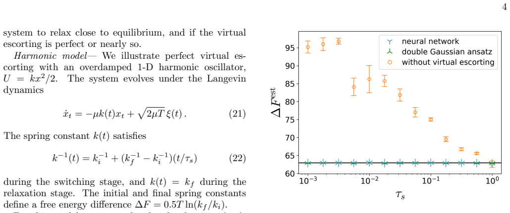
Asλvaries from 0 to 1, these minima approach one another, coalescing at the origin. For this process, ∆F= 62.94· · ·atT= 1 [29]. This model process illustrates the poor convergence of Eq. 1 [29], and the efficiency gains that can be achieved with escorting [4]. Here, we use it to illustrate virtual escorting, whenρ(x, t) is not known analytically. FIG. 2....
-
[2]
Jarzynski, Phys
C. Jarzynski, Phys. Rev. Lett.78, 2690 (1997)
1997
-
[3]
Jarzynski, Phys
C. Jarzynski, Phys. Rev. E56, 5018 (1997)
1997
-
[4]
Vaikuntanathan and C
S. Vaikuntanathan and C. Jarzynski, Europhys. Lett.87, 60005 (2009)
2009
-
[5]
Vaikuntanathan and C
S. Vaikuntanathan and C. Jarzynski, Phys. Rev. Lett. 100, 190601 (2008)
2008
-
[6]
Wirnsberger, A
P. Wirnsberger, A. J. Ballard, G. Papamakarios, S. Aber- crombie, S. Racani` ere, A. Pritzel, D. Jimenez Rezende, and C. Blundell, J. Chem. Phys.153, 144112 (2020)
2020
-
[7]
Vargas, S
F. Vargas, S. Padhy, D. Blessing, and N. N¨ usken, in International Conference on Learning Representations (ICLR)(2024)
2024
-
[8]
Zhong, B
A. Zhong, B. Kuznets-Speck, and M. R. DeWeese, Phys. Rev. E110, 034121 (2024)
2024
-
[9]
M´ at´ e, F
B. M´ at´ e, F. Fleuret, and T. Bereau, J. Phys. Chem. Lett.15, 11395 (2024)
2024
-
[10]
M´ at´ e, F
B. M´ at´ e, F. Fleuret, and T. Bereau, J. Chem. Phys.162, 124107 (2025)
2025
-
[11]
J. L. Rosa-Ra´ ıces and D. T. Limmer, J. Chem. Theory Comput.21, 11455 (2025)
2025
-
[12]
J. He, Y. Du, F. Vargas, Y. Wang, C. P. Gomes, J. M. Hern´ andez-Lobato, and E. Vanden-Eijnden, inAdvances in Neural Information Processing Systems (NeurIPS) (2025)
2025
-
[13]
Holdijk, N
L. Holdijk, N. M. Anand, M. M. Bronstein, and M. Welling, inInternational Conference on Learning Representations (ICLR)(2026)
2026
-
[14]
Schebek, J
M. Schebek, J. He, E. Hoffmann, Y. Du, F. No´ e, and J. Rogal, J. Chem. Phys.164, 184111 (2026)
2026
-
[15]
Sohl-Dickstein, E
J. Sohl-Dickstein, E. A. Weiss, N. Maheswaranathan, and S. Ganguli, inInternational Conference on Machine Learning (ICML)(2015)
2015
-
[16]
Y. Song, J. Sohl-Dickstein, D. P. Kingma, A. Kumar, S. Ermon, and B. Poole, inAdvances in Neural Infor- mation Processing Systems (NeurIPS)(2021)
2021
-
[17]
Albergo, N
M. Albergo, N. M. Boffi, and E. Vanden-Eijnden, J. Mach. Learn. Technol.26, 1 (2025)
2025
-
[18]
Risken, inThe Fokker-Planck equation: methods of solution and applications(Springer, 1989)
H. Risken, inThe Fokker-Planck equation: methods of solution and applications(Springer, 1989)
1989
-
[19]
Zwanzig,Nonequilibrium Statistical Mechanics(Ox- 6 ford University Press, 2001)
R. Zwanzig,Nonequilibrium Statistical Mechanics(Ox- 6 ford University Press, 2001)
2001
-
[20]
C. W. Gardineret al.,Handbook of Stochastic Methods (Springer, 1985)
1985
-
[21]
potential
In the context of overdamped Langevin dynamics, we refer toU(x, t) as a “potential” rather than using the more general term “energy function”
-
[22]
J. L. W. V. Jensen, Acta Mathematica30, 175 (1906)
1906
-
[23]
The Fisher divergence is also known as the relative Fisher information, the score- matching divergence, and the Hyv¨ arinen divergence
Explicitly,D KL(f||g)≡ R fln(f /g) andD F(f||g)≡ (1/2) R f|∇ln(f /g)| 2. The Fisher divergence is also known as the relative Fisher information, the score- matching divergence, and the Hyv¨ arinen divergence. It differs from (but is related to) the Fisherinformation, which involves derivatives with respect to auxiliary pa- rameters (e.g.θ) rather than sta...
-
[24]
X. Ding, H. T. Quan, and Y. Tu, (2026), arXiv:2606.17252
work page internal anchor Pith review Pith/arXiv arXiv 2026
-
[25]
Hyv¨ arinen and P
A. Hyv¨ arinen and P. Dayan, J. Mach. Learn. Res.6 (2005)
2005
-
[26]
Y. Song, S. Garg, J. Shi, and S. Ermon, inUncertainty in Artificial Intelligence Conference (UAI)(2020)
2020
-
[27]
R. W. Zwanzig, J. Chem. Phys.22, 1420 (1954)
1954
-
[28]
(4) asW[x t] = ∆U(x f , xi)−R τ 0 dt˙xt ◦∂ xU(x t, t), especially whenτ s ∼10 −3
We found that the numerical evaluation ofWwas im- proved by rewriting Eq. (4) asW[x t] = ∆U(x f , xi)−R τ 0 dt˙xt ◦∂ xU(x t, t), especially whenτ s ∼10 −3
-
[29]
Efron,The Jackknife, the Bootstrap, and Other Resampling Plans(Society for Industrial and Applied Mathematics (SIAM), 1982)
B. Efron,The Jackknife, the Bootstrap, and Other Resampling Plans(Society for Industrial and Applied Mathematics (SIAM), 1982)
1982
-
[30]
Oberhofer, C
H. Oberhofer, C. Dellago, and P. L. Geissler, J. Phys. Chem. B109, 6902 (2005)
2005
-
[31]
Gaussian Error Linear Units (GELUs)
D. Hendrycks and K. Gimpel, (2016), arXiv:1606.08415
work page internal anchor Pith review Pith/arXiv arXiv 2016
-
[32]
D. P. Kingma and J. Ba, inInternational Conference on Learning Representations (ICLR)(2015)
2015
-
[33]
Frenkel and A
D. Frenkel and A. J. Ladd, J. Chem. Phys81, 3188 (1984)
1984
-
[34]
Lipman, R
Y. Lipman, R. T. Q. Chen, H. Ben-Hamu, M. Nickel, and M. Le, inInternational Conference on Learning Rep- resentations (ICLR)(2023)
2023
-
[35]
Klinger and G
J. Klinger and G. M. Rotskoff, Phys. Rev. E111, 014114 (2025)
2025
-
[36]
Ikeda, T
K. Ikeda, T. Uda, D. Okanohara, and S. Ito, Phys. Rev. X15, 031031 (2025)
2025
-
[37]
(13),∇ ·u θ =µT∇ 2Sθ −µ∇ 2U
In Eq. (13),∇ ·u θ =µT∇ 2Sθ −µ∇ 2U
-
[38]
Seifert, Rep
U. Seifert, Rep. Prog. Phys.75, 126001 (2012)
2012
-
[39]
Peliti and S
L. Peliti and S. Pigolotti,Stochastic Thermodynamics: An Introduction(Princeton University Press, 2021)
2021
-
[40]
D. T. Limmer,Statistical Mechanics and Stochastic Ther- modynamics(Oxford University Press, 2024)
2024
-
[41]
Seifert,Stochastic Thermodynamics(Cambridge Uni- versity Press, 2025)
U. Seifert,Stochastic Thermodynamics(Cambridge Uni- versity Press, 2025)
2025
-
[42]
B. D. Anderson, Stoch. Process. Their Appl.12, 313 (1982)
1982
-
[43]
J. Ho, A. Jain, and P. Abbeel, inAdvances in Neural Information Processing Systems (NeurIPS)(2020)
2020
-
[44]
Y. Wang, L. Herron, and P. Tiwary, Proc. Natl. Acad. Sci. U.S.A.119, e2203656119 (2022)
2022
-
[45]
M. Xu, L. Yu, Y. Song, C. Shi, S. Ermon, and J. Tang, inInternational Conference on Learning Representations (ICLR)(2022)
2022
-
[46]
In the DM literature the result traces back to rigorous mathematical analysis [41]
We have derived this result using standard tools of nonequilibrium statistical physics and stochastic thermo- dynamics [37–40]. In the DM literature the result traces back to rigorous mathematical analysis [41]
-
[47]
Hummer and A
G. Hummer and A. Szabo, Proc. Natl. Acad. Sci. U.S.A. 98, 3658 (2001)
2001
-
[48]
Hummer and A
G. Hummer and A. Szabo, Acc. Chem. Res.38, 504 (2005)
2005
-
[49]
Ge and D.-Q
H. Ge and D.-Q. Jiang, J. Stat. Phys.131, 675 (2008)
2008
-
[50]
Note that the sumv θ +u θ describes Hamiltonian flow with friction under the HamiltonianH(x, t)
-
[51]
time-reversed
X. Glorot, A. Bordes, and Y. Bengio, inInternational Conference on Artificial Intelligence and Statistics (AIS- TATS)(2011). 7 Appendix A: Virtual escorted free energy estimation and diffusion models The efficacy of virtual escorted free energy estimation (VE for short) hinges on the ability to infer, up to normal- ization, a time-dependent density,ρ(x, t...
2011
-
[52]
imperfect
Explicit Construction ofL θ Given a choice ofπ θ(x, t), the validity of Eq. (B11) for Hamiltonian or underdamped Langevin dynamics requires an operatorL θ that satisfies Eqs. (B4) and (B6), for some fielduθ, whereLin Eq. (B6) is the evolution operator governing the unescorted evolution. We now constructL θ explicitly, for the underdamped Langevin case. Th...
discussion (0)
Sign in with ORCID, Apple, or X to comment. Anyone can read and Pith papers without signing in.