REVIEW 3 major objections 3 minor 3 references
Contextual Slate GLM Bandits with Limited Adaptivity
T0 review · 3 major / 3 minor · reviewed 2026-08-04 · deepseek-v4-flash
Pith's one-line read Contextual slate bandits with GLM rewards can match fully adaptive regret using only O(log log T) or O(Nd log T) policy updates, under a diversity condition.
desk verdict New algorithms and a clever scaling-slate trick, but the central eigenvalue-growth lemma is false and the κ-free regret bounds are not established as written. read the letter →
The pith
A machine-rendered reading of the paper's core claim, the machinery that carries it, and where it could break.
The reading
What carries the argument
The load-bearing construction is the slot-level scaled design matrix H_i = λI + Σ_t ˙μ(b_t^T θ̂_0) β_t^{-1} x_t^i (x_t^i)^T, where b_t is the 'scaling slate'—the item in each slot with largest norm under the warm-up inverse design matrix—and β_t is an exponential self-concordance normalizer. This matrix plays two roles: it upper and lower bounds the full slate-level design and the Hessian of the GLM log-likelihood, so the MLE confidence ellipsoid transfers from Nd dimensions to per-slot d dimensions; and the scaling-slate ratio ˙μ(b_t^T θ̂_0)/˙μ(x_t^T θ̂_0) is O(1), which cancels the κ factor that normally appears in GLM regret. Around this, the algorithms use G-optimal designs—probability d
What would settle it
Run B-SlateGLinCB or RS-SlateGLinCB on item distributions with zero conditional mean but rank-deficient or anisotropic conditional covariance—for example, every item in one slot lies in a fixed low-dimensional subspace—and record the minimum eigenvalue of each slot's H_i at every batch or update. The proof requires λ_min(H_i) ≥ λ + (ρ/2)t after t rounds; if growth flattens below that slope, the diversity assumption is violated and the regret bounds no longer apply. A simpler check: construct a distribution with nonzero conditional mean, which already breaks the zero-mean half of Assumption 2.1
Extended reading notes
Core claim
The central claim is that in the slate GLM bandit setting, limited adaptivity is compatible with state-of-the-art regret. Under a diversity assumption on the item sequences, B-SlateGLinCB partitions the horizon into O(log log T) batches and attains regret Õ(RS N d^{3/2} sqrt(T E_{X~D} μ'(x_*^T θ*))), while RS-SlateGLinCB makes only O(Nd log T) adaptive parameter updates and attains regret Õ(R sqrt(T) + R S^{1/2} N d sqrt(Σ_t μ'(x_{t,*}^T θ*))). Both bounds match the rate of the fully adaptive slate GLM algorithm and, crucially, have leading terms free of κ—the instance-dependent non-linearity parameter that can be exponential in the parameter norm in ordinary GLM bandit bounds. The authors e
Load-bearing premise
The load-bearing premise is the diversity assumption (Assumption 2.1): for each slot, the item actually selected, conditioned on past rounds, must have zero mean and covariance at least ρI in every direction; the paper does not prove that G-optimal sampling enforces this. If the environment violates it, the linear-eigenvalue-growth lemmas fail and both regret bounds collapse.
Editorial extensions
If this is right
- Batched deployment becomes practical: only O(log log T) policy updates give regret Õ(N d^{3/2} sqrt(T)), and rounds within a batch can run in parallel.
- Rarely-switching deployment cuts optimization cost: O(Nd log T) parameter refits give regret Õ(N d sqrt(T)), matching a fully adaptive policy that updates every round.
- The κ-free leading term removes an exponential-in-S penalty that typically appears in GLM bandit bounds, so the guarantees remain meaningful for strongly nonlinear reward links.
- Slot-wise G-optimal sampling keeps per-round time polynomial in N despite an action space of size 2^{Ω(N)} slates.
- The paper's heuristic variant B-SlateGLinCB+ matches the fully adaptive baseline empirically on prompt exemplar selection; proving its bounds would give the practical version a theorem as well.
Reading between the lines
- One testable extension is to replace the diversity assumption with a forced-exploration mechanism: if the algorithm actively samples items covering low-eigenvalue directions, the eigenvalue-growth lemmas could be proven rather than assumed, broadening applicability.
- The same scaling-slate trick—using a worst-case normalizing item to bound the link-function ratio—may transfer to other structured bandits with GLM rewards, such as multi-slot ranking or assortment problems, and would likely remove κ from their leading regret terms.
- The empirical advantage of pruning only against the most recent batch (B-SlateGLinCB+) suggests that multi-batch elimination is conservative; a regret proof for that variant could yield both faster algorithms and tighter constants.
- Because the bounds depend on E[μ'(x_*^T θ*)] at the optimal slate, the algorithms may adapt to easy instances automatically; an experiment varying the separability of the optimal slate could test whether this instance-dependence is real or an artifact of the analysis.
Signed reviews
Editorial analysis
A structured set of objections, weighed in public.
Referee Report
Summary. The paper studies contextual slate bandits with generalized linear model (GLM) rewards under two limited-adaptivity regimes. It proposes B-SlateGLinCB, which operates in O(log log T) batches, and RS-SlateGLinCB, which makes only O(Nd log T) parameter updates. Under a diversity assumption on the selected items (Assumption 2.1), the paper claims regret bounds of tilde-O(N d^{3/2} sqrt(T E[\dot{\mu}(x_*^T \theta_*)])) for the batched algorithm and tilde-O(R sqrt(T) + R S^{1/2} N d sqrt(sum_t \dot{\mu}(x_{t,*}^T \theta_*))) for the rarely-switching algorithm, both with leading terms independent of the nonlinearity parameter kappa. The algorithms select slotted items independently to avoid exponential slate enumeration, and the paper includes synthetic experiments, a prompt-tuning application, and an empirical check of eigenvalue growth.
Significance. If the theoretical results were correct, they would be a valuable advance: they would bring the limited-adaptivity toolkit to slate bandits with GLM feedback, achieve computationally efficient poly(N) per-round selection, and match the regret of the fully adaptive Slate-GLM-OFU while removing the kappa-dependence that afflicts many GLM bandit bounds. The algorithmic ideas are reasonable and the empirical comparisons are suggestive. However, the central proof mechanism—linear growth of eigenvalues of the scaled design matrices—rests on a false generalization of a martingale lemma, and the diversity assumption is not shown to hold for the algorithms' own selection rules. The main theoretical claims are therefore not established in this version.
major comments (3)
- [Appendix D, Lemma D.1] Lemma D.1 is false as stated. In the proof, after obtaining |sum x_s x_s^T - t Sigma_C| <= (1-c)rho t, the text concludes lambda_min(sum x_s x_s^T) >= t lambda_min(Sigma_C) - (1-c)rho t >= alpha rho t - (1-c)rho t >= c rho t. The last inequality would require alpha >= 1, but the lemma allows alpha in (0,1]. The correct conclusion is lambda_min >= gamma + (alpha+c-1)rho t, which may be negative and is at best gamma + c' alpha rho t. This is not a minor slip: Lemmas A.12, A.13, C.9, and C.10 apply this lemma with alpha = kappa^{-1} beta_t^{-1} (or kappa^{-1} e^{-1}) and rely on the claimed linear rate lambda + rho |T|/2. Without that rate, the multiplicative equivalence and the norm bound ||x||_{H^{-1}} <= 2 sum ||x^i||_{(H^i)^{-1}} fail, and with them the regret bounds in Theorems 3.1 and 4.1.
- [Section 2.5, Assumption 2.1] Assumption 2.1 is stated as though the algorithm guarantees diversity of the selected items, but no such guarantee is proved. In B-SlateGLinCB (Algorithm 1, Step 22) the item x_t^i is sampled from a G-optimal design on X_t^i; the distribution pi_G(X_t^i) generally has nonzero mean, so E[x_t^i | F_{t-1}] = 0 need not hold. In RS-SlateGLinCB (Algorithm 2, Step 5/17) the selection is deterministic given X_t^i and the current matrices, again with no reason to be conditionally zero-mean. Since the regret proofs invoke Assumption 2.1 for the algorithm's own sequence, the results apply only to a special class of environment selections that is not characterized. The paper should either prove the assumption for its algorithms under explicit conditions on D^i, or restate it as a separate structural condition and check it for the item-set distributions used in the experiments.
- [Appendix A.5, Lemma A.12] The application of the diversity assumption to the scaled vectors is not justified. The scaled vector is \bar{x}_t^i = sqrt(\dot{\mu}(b_t^T \hat{\theta}_0)/\beta_t) x_t^i, where b_t and \beta_t depend on the current item set X_t^i and are not measurable with respect to F_{t-1}. The displayed inequality E[\bar{x}_t^i \bar{x}_t^i^T | F_{t-1}] = E[\dot{\mu}(b_t^T \hat{\theta}_0)\beta_t^{-1} x_t^i x_t^i^T | F_{t-1}] \succeq \rho \kappa^{-1} \beta_t^{-1} I treats \beta_t as a fixed constant; in reality the best deterministic bound is \beta_t \le e^{2S}, yielding an exponentially small \alpha = \kappa^{-1} e^{-2S}. Combined with the error in Lemma D.1, this reintroduces the kappa-dependence that the paper claims to eliminate, so the kappa-free statement is unsupported.
minor comments (3)
- [Section 5] The experimental figures report averages over 25 seeds but no error bars or confidence intervals, making it hard to assess the statistical significance of the comparisons, especially when the claimed advantage over baselines is modest.
- [Appendix C.1 vs Algorithm 2] The notation section defines lambda = O(R sqrt(NdS log(ST/delta^-1))), while Algorithm 2 initializes lambda = O(NdR^2 S^{-1} log(T delta^-1)). These are inconsistent; the correct value used in the proofs should be stated clearly.
- [Throughout] Several small presentation issues: 'Kiefer-Wolfowitz' is misspelled 'Keifer-Wolfowitz' in Section 2.7; 'Cauchy-Schwartz' appears in Appendix B instead of 'Cauchy-Schwarz'; reference [KRS] lacks a venue/year; and the proof of Lemma A.8 relies on 'Claim A.8 from [SDBS24]' without restating it, which hinders verification.
Circularity Check
κ-free leading terms flow through Lemma D.1's boundary-case substitution (rate cρt only at α=1, applied with α=κ^{-1}β_t^{-1}); no fitted or definitional circularity elsewhere.
-
other
[Appendix D, Lemma D.1 (proof); applied in Lemmas A.12 and C.9 (Appendices A.5, C.4)]
"λmin(Ps∈[t] xsx⊤s) ≥ tλmin(ΣC) − (1−c)ρt ≥ αρt− (1−c)ρt ≥ cρt where the last inequality uses the fact that α∈(0,1] ... Applying Lemma D.1 using the quantities α=κ−1β−1t (≤1), ... and c=0.5 ... λmin(λI+Ps∈[t] xi sxi s⊤) ≥ λ+ρt/2"
The chain αρt−(1−c)ρt ≥ cρt holds only if αρ ≥ ρ, i.e., at α=1; for α∈(0,1] the correct remainder is (α+c−1)ρt. The applications explicitly set α=κ^{-1}β_t^{-1}≤1 (κ≥1, β_t≥1) and c=0.5 yet conclude λ_min ≥ λ+ρt/2, importing the full κ-free rate ρ by the same α=1 boundary substitution rather than from Assumption 2.1 on the original x_t^i. The preceding 'diversity' equality also treats the random factor ˙µ(b_t^⊤θ0)/β_t as F_{t-1}-measurable although b_t uses the current X_t^i. Since Lemmas A.12/C.9 carry the multiplicative equivalence diag(H^i)≃H and hence the leading terms in Theorems 3.1/4.1 (and the 'strictly weaker than [GS25]' claim), the headline κ-independence reduces, by the paper's own inequality, to the α=1 boundary; corrected, the growth is (1/2)κ^{-1}β_t^{-1}ρt and κ reappears.
full rationale
No parameter is fitted to data and then reported as a prediction: the regret bounds are conditional on the explicitly stated Assumption 2.1 (a premise about the algorithm's own sequence, not an output), and B-SlateGLinCB+ is honestly labeled a heuristic with theory deferred (Appendix F: "leave the theoretical analysis of this algorithm as an interesting future direction"; Conclusions: "Developing batched algorithms with provably optimal regret guarantees ... remains an important future direction"). The self-citations ([GS25], [SDBS24], [MGS25], [DS24]) share authors with this paper and supply load-bearing technical lemmas (Lemma B.1/B.2/B.7/D.2 of [GS25], confidence sets and Claim A.8 of [SDBS24]); these are published, parameter-free results that do not themselves contain the limited-adaptivity slate claim, so under the reviewing rule they count as independent support rather than circularity. The one construction-level reduction I can exhibit is in the eigenvalue linear-growth lemma: Lemma D.1's own displayed inequality yields rate cρt only at the α=1 boundary, yet the main proofs invoke it with α=κ^{-1}β_t^{-1}≤1 and claim the full ρt growth. That is exactly the step that manufactures the κ-free leading terms; corrected, the growth is κ^{-1}β_t^{-1}-scaled and the claimed κ-independence in Theorems 3.1 and 4.1 collapses to a correctness/technical flaw at the derivation hinge. This is localized (no global equivalence of inputs and outputs, no forced self-citation chain), so the score is 5 rather than 6-10; the remaining issues (non-F_{t-1}-measurable scaling inside conditional expectations, the zero-mean half of Assumption 2.1 being unenforced) are better classed as correctness risks than as circularity.
Assumptions & free parameters
assumptions (7)
- domain assumption GLM reward model: rewards r∈[0,R] a.s., b twice differentiable, μ monotone and Lμ-Lipschitz, self-concordance |μ¨| ≤ R μ˙.
- domain assumption Unknown parameter norm bound ||θ*||_2 ≤ S with S known; each item norm ||z||_2 ≤ 1/√N.
- domain assumption Diversity Assumption 2.1: for all slots i, E[x_t^i | F_{t-1}] = 0 and E[x_t^i (x_t^i)^T | F_{t-1}] ⪰ ρ I for the algorithm-selected items.
- domain assumption For the batched setting, item sets X_t^i are sampled independently from a distribution D^i.
- standard math G-optimal designs exist and can be computed approximately in polynomial time; Kiefer-Wolfowitz bound holds.
- domain assumption GLM-MLE concentration inequalities (Lemma A.1 from [SDBS24]) hold with the stated λ and γ.
- standard math Matrix Freedman inequality and related martingale lemmas from [GS25] hold as stated.
Cite this review
Pith. "Pith review of Contextual Slate GLM Bandits with Limited Adaptivity." pith.science (2026). https://pith.science/paper/VSMK4E4M
@misc{pith2026260631449,
  author       = {Pith},
  title        = {Pith review of: Contextual Slate GLM Bandits with Limited Adaptivity},
  year         = {2026},
  howpublished = {\url{https://pith.science/paper/VSMK4E4M}},
  note         = {Machine review of arXiv:2606.31449}
}
abstract
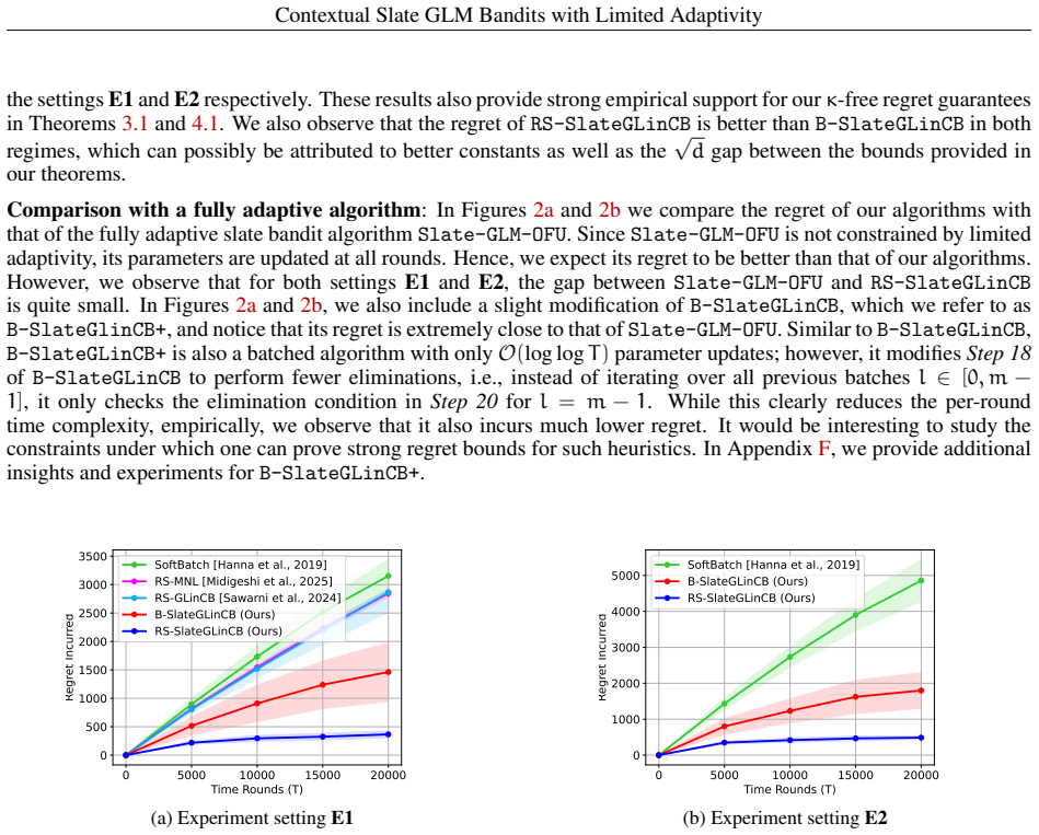
We investigate the contextual slate bandit problem with generalized linear rewards under limited adaptivity. At each round, the learner is presented with $N$ sets of items, where each item is represented by a $d$-dimensional feature vector. The learner then constructs a slate by selecting one item per set; the resulting slate yields a scalar reward sampled from a Generalized Linear Model (GLM). We propose algorithms under two limited-adaptivity settings: (a) Batched and (b) Rarely-Switching. For the batched setting, we introduce B-SlateGLinCB, which partitions the time horizon into $\mathcal{O}(\log\log T)$ batches such that each batch's policy relies only on data from previous batches. For the rarely-switching setting, we propose RS-SlateGLinCB, which adaptively performs only $\mathcal{O}(Nd\log T)$ parameter updates. Under a diversity assumption on the item sequences, we prove that B-SlateGLinCB and RS-SlateGLinCB achieve regret bounds of $\mathcal{O}(Nd^{3/2}\sqrt{T})$ and $\mathcal{O}(Nd\sqrt{T})$, respectively. Notably, both bounds are independent of the non-linearity parameter $\kappa$ that is typically found to scale the regret of GLM bandit algorithms. Our algorithms are computationally efficient, requiring only $\text{poly}(N)$ time per round despite $2^{\Omega(N)}$ possible slates. Simulations show our algorithms outperform existing baselines with limited adaptivity and remain competitive with Slate-GLM-OFU, a fully adaptive state-of-the-art algorithm. Notably, a slightly modified B-SlateGLinCB empirically matches this baseline. Finally, we demonstrate strong performance in a practical in-context example selection task for language models.
Figures


Figures from the paper (5 more)


Reference graph
Works this paper leans on
-
[3]
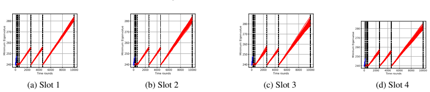
All the algorithms are run forT=10000for 50 different seeds for sampling rewards
We choose theℓ 2−norm ofθ ⋆ to beS=2. All the algorithms are run forT=10000for 50 different seeds for sampling rewards. We display the results forB-SlateGLinCBin Figure 6, forRS-SlateGLinCBin Figure 7, and forB-SlateGLinCB+ in Figure 8. Throughout, the black dotted lines represent the transition between batches (or in the case of RS-SlateGLinCB, the end o...
2000
-
[5]
Here,c 1 measures the N-gram similarity between the query and the example sentence
We describe them in greater detail here.jdenotes the joint embedding of the queryq t and the candidate example eik t ,lis the example’s label, i.e,l=l ik t , andc= (c 1, c2)represents a pair of scores that measure the similarity between the query and the example. Here,c 1 measures the N-gram similarity between the query and the example sentence. This is d...
-
[150]
We run the algorithms forT∈{5000, 10000, 15000, 20000}and display the results in Figure 5d. In Figure 5, we see that the gap betweenRS-SlateGLinCBandSlate-GLM-OFUis very small, even though we would expectSlate-GLM-OFUto have much better regret because of its fully sequential nature. However, there remains a significant gap between the regrets incurred byB...
Reviewed August 4, 2026 · model on record in the stance chip above.
Discussion (0). Continue with ORCID to comment.