REVIEW 2 major objections 7 minor 46 references
An Efficient Method for Gibbs Free Energy Evaluation under Volume Compression
T0 review · 2 major / 7 minor · reviewed 2026-07-10 · glm-5.2
Pith's one-line read Three phonon calculations replace twenty for pressure-temperature phase diagrams
desk verdict Practical interpolation method that cuts QHA phonon calculations from ~20 to 3 volumes, validated well but with a selection-circularity caveat. read the letter →
The pith
A machine-rendered reading of the paper's core claim, the machinery that carries it, and where it could break.
The reading
What carries the argument
The method operates by first selecting three stable volumes bracketing the equilibrium volume path traversed during Gibbs minimization. At these sparse volumes, full phonon calculations yield frequencies, ZPE, and static energies. The ZPE-level effective Grüneisen parameter is extracted as a through-origin slope of ln[ZPE(V)/ZPE(V0)] versus ln(V0/V). For each phonon mode j, a local Grüneisen slope is computed between each pair of adjacent sparse volumes. Target-volume frequencies are reconstructed by exponential interpolation: omega_j(V_m) = omega_j(V_a) * exp[gamma_j * (ln(V0/V_m) - ln(V0/V_a))]. Only positive-frequency modes enter the sums; imaginary or zero frequencies are discarded. The
What would settle it
Find a system where, within the moderate compression range (above 0.8*V0), a phonon mode undergoes a crossing or softening between two sparse volume endpoints such that the linear log-volume interpolation produces a qualitatively wrong frequency at an intermediate volume, leading to a Gibbs free energy error large enough to flip an assigned stable phase. The Ta2O5 lambda phase, with 17.5 meV/atom MAE, already hints that such failures occur for complex polymorphs.
Extended reading notes
Core claim
The central finding is that the volume dependence of phonon frequencies in crystalline solids is smooth enough in the logarithmic volume coordinate that a piecewise mode-resolved Grüneisen interpolation using only three explicit phonon calculations can reconstruct Gibbs free energies to within sub-meV-per-atom accuracy for moderate compression ranges. The key object is the mode-resolved local Grüneisen slope, defined between two sparse volume endpoints for each phonon mode individually, which captures the mode-specific frequency shift without requiring a single global scaling parameter. Combined with a separate ZPE-level effective Grüneisen parameter for the static branch, this two-tiered重建y
Load-bearing premise
The method assumes that within a moderate compression range, phonon frequencies vary smoothly enough with the logarithm of volume that a locally linear Grüneisen slope between two sparse endpoints can faithfully reconstruct intermediate frequencies for every mode. This breaks down when mode crossings, soft modes, or incipient structural transformations within the interpolation interval change the topology of the phonon spectrum in ways that two endpoint frequencies cannot捕获.
Editorial extensions
If this is right
- High-throughput materials discovery pipelines that currently stop at zero-temperature energy ranking could add finite-temperature and finite-pressure phase stability checks at roughly one-seventh the phonon calculation cost, making thermodynamic validation of AI-generated crystal structures tractable at scale.
- The piecewise mode-resolved Grüneisen slopes themselves serve as a compact diagnostic: phases with large extracted gamma values flag strong volume sensitivity of specific modes, identifying candidates where denser sampling or explicit anharmonic treatment may be needed before running full calculations.
- The three-point framework extends naturally to more sparse volumes when higher accuracy is required, providing a tunable accuracy-cost tradeoff rather than a fixed-cost method.
- For systems where the method fails (strong compression, soft modes, mode crossings), the failure is detectable: the rapid error growth beyond 0.8*V0 shown in Figure 12 provides a quantitative criterion for when to switch to full dense-volume QHA.
Editorial analysis
A structured set of objections, weighed in public.
Referee Report
Summary. The manuscript presents a sparse-volume Grüneisen interpolation (GI) method for reconstructing Gibbs free energies under volume compression. The approach calculates phonon spectra at only 3 selected volumes and reconstructs the full free energy surface using a ZPE-level effective Grüneisen parameter for the static-ZPE branch and piecewise mode-resolved Grüneisen slopes for the finite-temperature vibrational branch. The method is validated against dense-grid QHA benchmarks for 7 systems (C, Al, Si, Ge, TiO2, PtO2, Ta2O5), achieving sub-0.53 meV/atom MAE for the six simpler systems and 5.9-9.0x speedup, while preserving phase-stability topology for the complex Ta2O5 polymorphs.
Significance. The paper addresses a genuine computational bottleneck in high-throughput materials discovery: the cost of dense-volume QHA phonon calculations for finite-temperature phase-diagram construction. The mathematical formulation (Eqs. 8-13) is internally consistent and builds on the standard Grüneisen relation. The validation is systematic, with explicit MAE metrics at both ZPE and Gibbs levels, pointwise error maps, phase-diagram comparisons, and thermal-expansion coefficient recovery. The honest reporting of breakdown for Ta2O5 (MAE up to 17.5 meV/atom) and the applicable compression range (Fig. 12) is commendable. The comparison with the VIP method (Appendix B) provides useful context. The speedup factors are practically significant for the materials discovery pipeline described in the introduction.
major comments (2)
- Section II.A, Eq. (14): The sparse-volume selection procedure uses the dense QHA reference to determine V_eq(P,T) and identify the volume range traversed by the equilibrium path. The three sparse phonon points are then chosen to bracket this QHA-derived path. This creates a practical circularity in the headline speedup claim: the method requires knowledge of the expensive QHA calculation it claims to replace in order to select its own input points. The sensitivity tests mentioned in Section II.A ('we repeat the calculation for available three-point combinations satisfying this local bracket condition') and Appendix Fig. A4 only vary combinations within the QHA-defined bracket, not selections made without QHA knowledge. In a real deployment scenario, one would not have the dense QHA reference and would need to select sparse volumes from cheaper proxies (static EOS, or 1-2 exploratory phon
- The abstract states speedups of '5.911-9.023 times' relative to QHA workflows. However, as noted above, the sparse-point selection itself requires the QHA V_eq(P,T) path (Eq. 14). If the selection cost is included, the effective speedup is smaller. The paper should either (a) demonstrate that proxy-based selection (e.g., using static EOS or a single exploratory phonon point to estimate the relevant volume range) yields comparable MAEs, or (b) explicitly state that the reported speedup assumes the sparse points are selected without the full QHA reference, and provide a practical protocol for doing so. Without this, the speedup claim is conditional on information that would not be available in the intended use case.
minor comments (7)
- Table I: The R² values for Si (0.887) and Al (0.981) are notably lower than for other systems (0.999 for C, 0.998 for Ge). Given that Al and Si are among the systems with larger MAE_G values (0.52 and 0.19 meV/atom respectively), a brief discussion of whether the lower R² is correlated with the reconstruction error would strengthen the analysis.
- Section II.A, Eq. (12): The notation uses subscripts a and b for sparse-volume endpoints, but the text also uses i for sparse volumes in general. Clarifying that a and b are specific instances of i would help readers.
- Section III.C: The Ta2O5 errors range up to 17.5 meV/atom for the lambda phase. While the paper notes this is due to 'phase-specific soft modes, mode crossings, and shallow free energy separations,' it would be useful to specify which phases have known soft modes or mode crossings in the studied pressure range, to help users assess applicability.
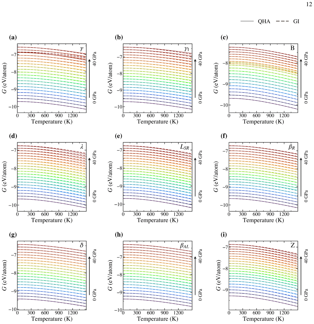
- Fig. 3: The pressure ranges are indicated outside each panel but are difficult to read. Consider using matching colors/symbols for pressure labels and curves, or adding a legend.
- Section II.A, Eq. (15): The treatment of imaginary/zero-frequency modes (simple discarding) is stated without justification. For systems near dynamical instability, this could introduce non-negligible errors. A brief comment on the magnitude of this approximation, especially for the Ta2O5 phases where some may be near stability boundaries, would be valuable.
- The abstract states speedups with excessive precision (5.911-9.023x). Rounding to 5.9-9.0x would be more appropriate for the abstract.
- Reference [39] is cited as 'arXiv:2602.03649; Phys. Rev. B (in press).' If now published, the reference should be updated.
Circularity Check
Mild benchmark-setup circularity in sparse-point selection (Eq. 14), but the GI derivation is self-contained and independently valid.
-
fitted input called prediction
[Section II.A, Eq. 14 and surrounding text]
"For a target pressure-temperature window, we first determine V_eq(P,T) = argmin_V [F_QHA(T,V) + PV] from the dense QHA reference and identify the range traversed by V_eq(P,T). ... Three adjacent or nearby stable volumes are then chosen to bracket the local V_eq(P,T) path"
The 3 sparse phonon volumes used for GI reconstruction are selected using the dense QHA V_eq(P,T) path. The MAE is then measured against that same QHA benchmark. This creates a mild benchmark circularity: the interpolation points are optimally placed using knowledge from the calculation the method claims to replace. However, the paper mitigates this by noting 'In broad compression benchmarks where the target window spans the full stable interval, this procedure reduces to using representative low-, middle-, and high-volume points,' meaning the simple benchmark systems (C, Al, Si, Ge, TiO2, PtO2) do not actually require QHA-informed selection. The Ta2O5 case, which does use QHA-informed selection, shows larger errors. The GI interpolation method itself (Eqs. 8-13) is a legitimate scheme not
full rationale
The core derivation chain is not circular. The Grüneisen relation (Eq. 8) is a standard physics identity. The ZPE-level scaling (Eq. 11) and mode-resolved slopes (Eq. 12) are extracted from sparse data and applied as interpolation — they do not presuppose the target result. The Gibbs free energy reconstruction (Eq. 13) assembles these pieces without definitional circularity. The one concern is Eq. 14: sparse-point selection uses the dense QHA V_eq path, creating a mild benchmark-setup circularity where the method's accuracy is evaluated under optimal point placement informed by the benchmark itself. However, the paper explicitly states this reduces to simple low/mid/high selection for broad benchmarks, and the sensitivity tests (Fig. A4) show robustness within the bracket. The self-citation to Gong et al. [39] for Ta2O5 data is data sourcing, not a load-bearing theoretical claim. The method has substantial independent content and is validated against external benchmarks. Score 2 reflects the mild benchmark circularity without undermining the central claim.
Assumptions & free parameters
free parameters (3)
- gamma_ZPE =
system-dependent (e.g., 1.108 for C, 1.597 for Al, 0.512-2.026 for Ta2O5 phases)
- gamma_j^{ab} =
mode- and interval-dependent
- N_sp (number of sparse volumes) =
3
assumptions (4)
- domain assumption Phonon frequencies vary smoothly with logarithmic volume coordinate within moderate compression ranges, so local linear Grüneisen slopes are valid approximations.
- domain assumption Quasi-harmonic approximation (QHA) provides a valid benchmark for Gibbs free energies in the tested systems.
- ad hoc to paper Modes with imaginary or zero frequencies can be discarded from phonon sums without significant error.
- domain assumption Vibrational free energy is the dominant finite-temperature contribution for the tested nonmagnetic systems.
Cite this review
Pith. "Pith review of An Efficient Method for Gibbs Free Energy Evaluation under Volume Compression." pith.science (2026). https://pith.science/paper/G7E3BCCO
@misc{pith2026260708608,
  author       = {Pith},
  title        = {Pith review of: An Efficient Method for Gibbs Free Energy Evaluation under Volume Compression},
  year         = {2026},
  howpublished = {\url{https://pith.science/paper/G7E3BCCO}},
  note         = {Machine review of arXiv:2607.08608}
}
read the original abstract
Accurate evaluation of Gibbs free energies is essential for constructing pressure-temperature phase diagrams. Conventional methods based on the quasi-harmonic approximation (QHA) require phonon spectra at many volume points and are therefore expensive in general. Here we develop an efficient method based on the interpolation of a few ab initio data points for Gibbs free energy evaluation under volume compression. Phonon spectra are calculated only at selected volumes. An effective Gruneisen parameter derived from the zero-point energy (ZPE) reconstructs the static-ZPE branch, while piecewise mode-resolved Gruneisen slopes reconstruct the finite-temperature vibrational branches on the target volume grids. The method is validated against QHA benchmarks for diamond (C), Al, Si, Ge, rutile TiO2, beta-PtO2, and Ta2O5 polymorphs. For simple benchmark systems (C, Al, Si, Ge, rutile TiO2, and beta-PtO2), the Gibbs free energy mean absolute errors (MAEs) relative to the QHA benchmarks remain below 0.53 meV/atom, with a six-system average of 0.148 meV/atom, while the number of explicit phonon volume points is reduced from about 20-21 to 3 in the lowest-cost implementation. For the more complex Ta2O5 polymorphs, the reconstructed free energies reproduce the main phase-stability topology despite larger phase-dependent errors. With reference to the QHA workflows, the interpolation method in this work achieves speedups of 5.911-9.023 times and remains reliable for moderate compression ranges where phonon frequencies vary smoothly with volume.
Figures


Figures from the paper (9 more)




Reference graph
Works this paper leans on
-
[1]
A.Merchant,S.Batzner,S.S.Schoenholz,M.Aykol,G.Cheon, and E. D. Cubuk, Nature624, 80 (2023)
work page 2023
- [2]
-
[3]
B. Deng, P. Zhong, K. Jun, J. Riebesell, K. Han, C. J. Bartel, and G. Ceder, Nat. Mach. Intell.5, 1031 (2023)
work page 2023
-
[4]
C. Zeni, R. Pinsler, D. Zügner,et al., Nature639, 624 (2025)
work page 2025
-
[5]
A. Jain, S. P. Ong, G. Hautier, W. Chen, W. D. Richards, S. Dacek, S. Cholia, D. Gunter, D. Skinner, G. Ceder, and K. A. Persson, APL Mater.1, 011002 (2013)
work page 2013
-
[6]
D. C. Wallace,Thermodynamics of Crystals(Wiley, New York, 1972)
work page 1972
-
[7]
B. Grabowski, T. Hickel, and J. Neugebauer, Phys. Rev. B76, 024309 (2007)
work page 2007
- [8]
Show all 46 references
-
[9]
C1, 6364 (2013)
J.Lee,S.-C.Lee,C.S.Hwang,andJ.-H.Choi,J.Mater.Chem. C1, 6364 (2013). 21 FIG. A5. Electronic density of states and electronic entropy of fcc Al along the thermal-expansion path. Panel (a) shows the electronic DOS𝐷[𝑉 eq (𝑇), 𝐸], whose vertical axis is given in units of states eV...
2013
-
[10]
A. T. Dinsdale, Calphad15, 317 (1991)
1991
-
[11]
Liu, Calphad82, 102580 (2023)
Z.-K. Liu, Calphad82, 102580 (2023)
2023
-
[12]
M.T.Dove,Introduction to Lattice Dynamics(CambridgeUni- versity Press, Cambridge, 1993)
1993
-
[13]
Chen, Annu
L.-Q. Chen, Annu. Rev. Mater. Res.32, 113 (2002)
2002
-
[14]
I.Steinbach,Model.Simul.Mater.Sci.Eng.17,073001(2009)
2009
-
[15]
R. M. Martin,Electronic Structure(Cambridge University Press, Cambridge, 2004)
2004
-
[16]
S.Baroni,S.deGironcoli,A.DalCorso,andP.Giannozzi,Rev. Mod. Phys.73, 515 (2001)
2001
-
[17]
V. V. Ladygin, P. Yu. Korotaev, A. V. Yanilkin, and A. V. Shapeev, Comput. Mater. Sci.172, 109333 (2020)
2020
-
[18]
Hashimoto, T
K. Hashimoto, T. Tanaka, and Y. Gohda, Phys. Rev. B111, 224309 (2025)
2025
-
[19]
Zhang, B
X. Zhang, B. Grabowski, F. Körmann, C. Freysoldt, and J. Neugebauer, Phys. Rev. B95, 165126 (2017)
2017
-
[20]
Grüneisen, Ann
E. Grüneisen, Ann. Phys.344, 257 (1912)
1912
-
[21]
Kresse and J
G. Kresse and J. Furthmüller, Phys. Rev. B54, 11169 (1996)
1996
-
[22]
G.KresseandJ.Furthmüller,Comput.Mater.Sci.6,15(1996)
1996
-
[23]
P. E. Blöchl, Phys. Rev. B50, 17953 (1994)
1994
-
[24]
Kresse and D
G. Kresse and D. Joubert, Phys. Rev. B59, 1758 (1999)
1999
-
[25]
J. P. Perdew, K. Burke, and M. Ernzerhof, Phys. Rev. Lett.77, 3865 (1996)
1996
-
[26]
K.Parlinski,Z.Q.Li,andY.Kawazoe,Phys.Rev.Lett.78,4063 (1997)
1997
-
[27]
H. J. Monkhorst and J. D. Pack, Phys. Rev. B13, 5188 (1976)
1976
-
[28]
Methfessel and A
M. Methfessel and A. T. Paxton, Phys. Rev. B40, 3616 (1989)
1989
-
[29]
Yang and Y
Y. Yang and Y. Kawazoe, Phys. Rev. Mater.2, 034602 (2018)
2018
-
[30]
Y.W.Tong,H.M.Tang,andY.Yang,Comput.Mater.Sci.230, 112482 (2023)
2023
-
[31]
I. P. Zibrov, V. P. Filonenko, M. Sundberg, and P.-E. Werner, Acta Crystallogr. Sect. B56, 659 (2000)
2000
-
[32]
Lett.110, 235502 (2013)
S.-H.Lee,J.Kim,S.-J.Kim,S.Kim,andG.-S.Park,Phys.Rev. Lett.110, 235502 (2013)
2013
-
[33]
N. C. Stephenson and R. S. Roth, Acta Crystallogr. Sect. B27, 1037 (1971)
1971
-
[34]
Fukumoto and K
A. Fukumoto and K. Miwa, Phys. Rev. B55, 11155 (1997)
1997
-
[35]
L. A. Aleshina and S. V. Loginova, Crystallogr. Rep.47, 415 (2002)
2002
-
[36]
Ramprasad, J
R. Ramprasad, J. Appl. Phys.94, 5609 (2003)
2003
-
[37]
Wilhelm, Sci
S.Anzellini,M.T.Wharmby,F.Miozzi,A.Kleppe,D.Daisen- berger, and H. Wilhelm, Sci. Rep.9, 15537 (2019)
2019
-
[38]
L. C. Kelsall, M. Peña-Alvarez, M. Martinez-Canales, J. Binns, P. Dalladay-Simpson, R. T. Howie, E. Gregoryanz, and C. J. Pickard, J. Chem. Phys.154, 174702 (2021)
2021
-
[39]
Y.Gong,H.Tang,Y.Yang,andY.Kawazoe,arXiv:2602.03649; Phys. Rev. B (in press)
-
[40]
Y. Z. Guo and J. Robertson, Appl. Phys. Lett.104, 112906 (2014)
2014
-
[41]
Y.Yang,O.Sugino,andY.Kawazoe,SolidStateCommun.195, 16 (2014)
2014
-
[42]
Y. S. Touloukian, R. K. Kirby, R. E. Taylor, and P. D. Desai, Thermophysical Properties of Matter: The TPRC Data Series, Vol. 12, Thermal Expansion: Metallic Elements and Alloys (IFI/Plenum, New York, 1975)
1975
-
[43]
Okada and Y
Y. Okada and Y. Tokumaru, J. Appl. Phys.56, 314 (1984)
1984
-
[44]
P. B. Allen, Mod. Phys. Lett. B34, 2050025 (2020)
2020
-
[45]
Masuki, T
R. Masuki, T. Nomoto, R. Arita, and T. Tadano, Phys. Rev. B 105, 064112 (2022)
2022
-
[46]
Science Data Bank,https://www.scidb.cn/
Reviewed July 10, 2026 · model on record in the stance chip above.
Discussion (0). Sign in to comment.