Evaluation of the Biot-Savart integral in electrostatic problems with non-uniform Dirichlet boundary conditions
Pith reviewed 2026-05-25 10:00 UTC · model grok-4.3
The pith
The electric field from a planar region with fixed non-uniform boundary potential equals a Biot-Savart circulation term plus a correction for angular potential changes inside the region.
A machine-rendered reading of the paper's core claim, the machinery that carries it, and where it could break.
Core claim
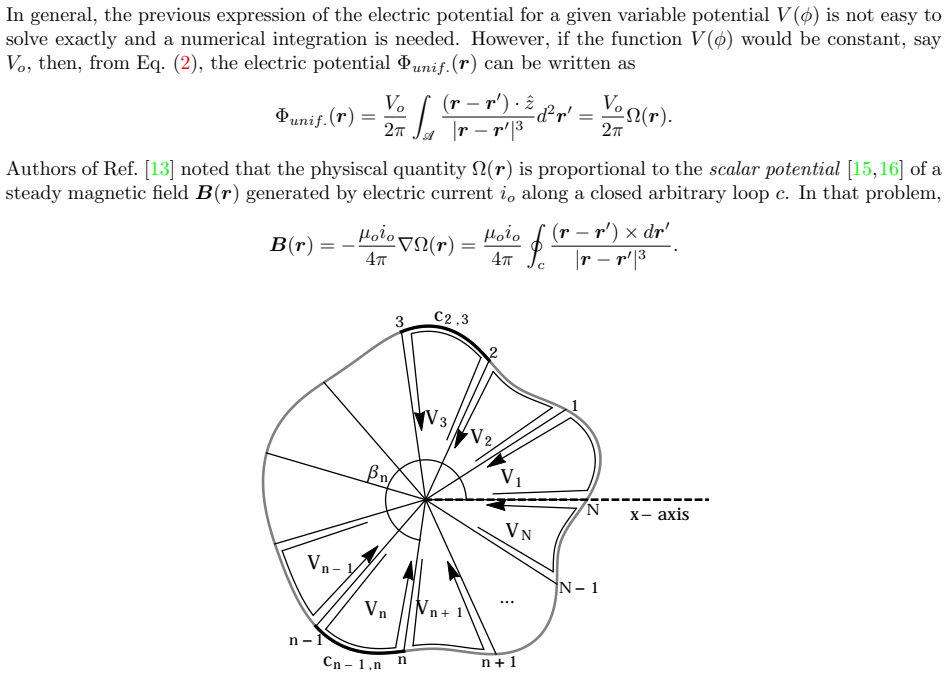
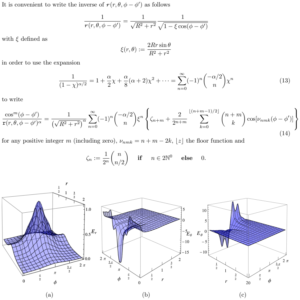
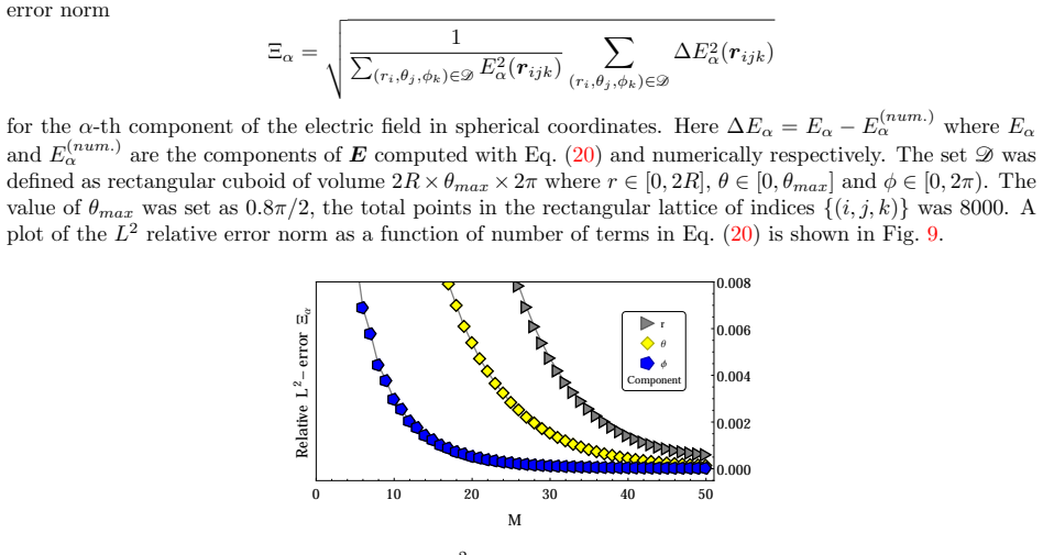
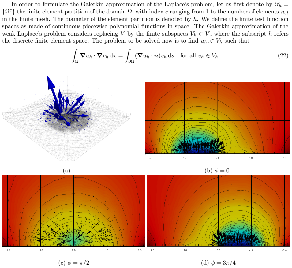
The electric field generated by a planar region A enclosed by contour c with fixed non-uniform potential is the sum of a term that depends on the circulation along c in the manner of the Biot-Savart law and a second term that captures the angular variations of the potential across A. This decomposition holds for any closed loop c. The method yields exact series solutions when the contour is a circle and the potential is fully periodic, and these agree with numerical computations and finite-element results.
What carries the argument
Decomposition of the electric field into a Biot-Savart-like circulation contribution from the boundary contour plus an angular-variation term inside the planar region.
If this is right
- Exact series expansions for the field become available for circular contours with periodic boundary potentials.
- The decomposition applies to any closed contour shape.
- The two-term expression matches both direct numerical integration and finite-element simulations.
- The field can be obtained from boundary circulation data and interior angular derivatives without solving the full boundary-value problem.
Where Pith is reading between the lines
- The split may simplify calculations in other planar potential problems such as steady heat conduction or incompressible flow.
- Numerical solvers could use the decomposition to accelerate field evaluation near prescribed-potential boundaries.
- The same angular term might generalize to three-dimensional surfaces if the circulation contribution is replaced by an appropriate surface integral.
- Laboratory measurements of the field near a conducting loop with spatially varying voltage would provide a direct experimental test.
Load-bearing premise
The electric potential is fixed only on the boundary contour while the interior region is perfectly planar and free of other charges or boundaries.
What would settle it
Compute the electric field at a test point inside an elliptical contour carrying a sinusoidal potential and check whether the sum of the Biot-Savart term and the angular-variation term exactly matches the solution of Laplace's equation.
Figures
read the original abstract
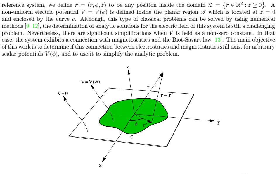
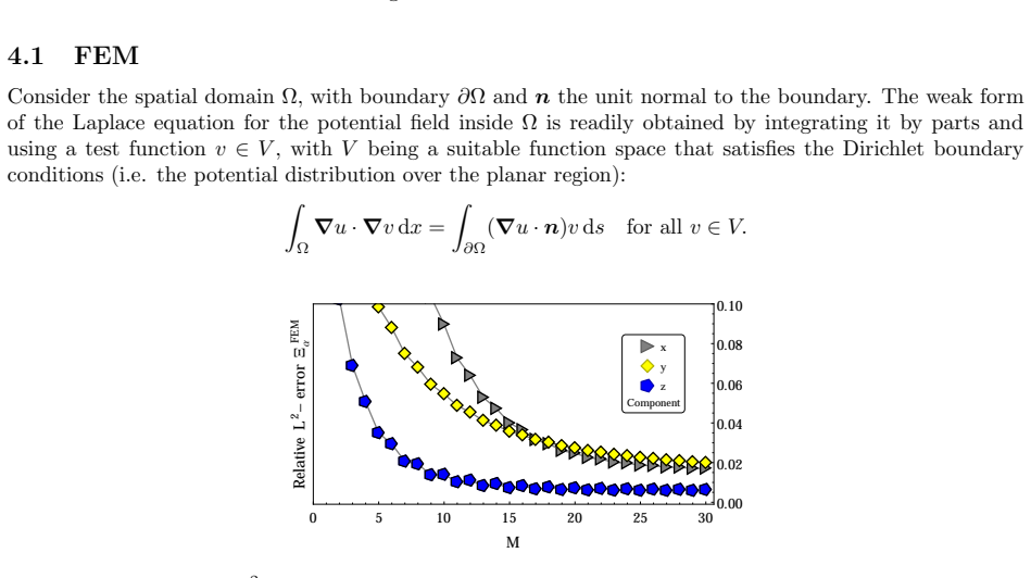
We present an analytical strategy to solve the electric field generated by a planar region $\mathcal{A}$ enclosed by a contour $c$ which is kept with a fixed but non-uniform electric potential. The approach can be used in certain situations where the electric potential on the space requires to solve the Laplace equation with non-uniform Dirichlet boundary conditions. We show that the electric field is due to a contribution depending on the circulation on the contour in a Biot-Savart way plus another one taking into account the angular variations of the potential in $\mathcal{A}$ valid for any closed loop $c$. The approach is used to find exact expansions solutions of the electric field for circular contours with fully periodic potentials. Analytical results are validated with numerical computations and the Finite Element Method. Keywords: Biot-Savart law, electrostatic problems, exactly solvable models.
Editorial analysis
A structured set of objections, weighed in public.
Referee Report
Summary. The manuscript proposes an analytical strategy for computing the electric field generated by a planar region A enclosed by a contour c held at a fixed but non-uniform electric potential. It decomposes the field into a Biot-Savart-like contribution from the circulation along c plus a term accounting for angular variations of the potential within A, asserting this split holds for any closed loop c. Explicit series expansions are derived for the special case of circular contours with fully periodic potentials; these are validated against direct numerical computations and the Finite Element Method.
Significance. If the general decomposition can be established rigorously, the method would supply exact, parameter-free solutions for a class of 2D electrostatic problems with non-uniform Dirichlet data, extending integral representations akin to Biot-Savart to potential theory and providing useful benchmarks for numerical codes.
major comments (1)
- [Abstract / general formulation] Abstract and general claim: the statement that the decomposition 'is valid for any closed loop c' is not accompanied by a general integral representation or proof. The manuscript supplies explicit series solutions and FEM validation exclusively for circular contours; no derivation is shown demonstrating that the same split satisfies Laplace's equation and the prescribed Dirichlet data on non-circular contours without extra curvature or surface terms.
Simulated Author's Rebuttal
We thank the referee for the careful reading and constructive feedback. We address the major comment below.
read point-by-point responses
-
Referee: [Abstract / general formulation] Abstract and general claim: the statement that the decomposition 'is valid for any closed loop c' is not accompanied by a general integral representation or proof. The manuscript supplies explicit series solutions and FEM validation exclusively for circular contours; no derivation is shown demonstrating that the same split satisfies Laplace's equation and the prescribed Dirichlet data on non-circular contours without extra curvature or surface terms.
Authors: We agree that the manuscript asserts validity for arbitrary closed contours but provides the explicit derivation and validation only for the circular case. The decomposition follows from representing the potential as a harmonic function whose gradient yields a Biot-Savart-type line integral along c (capturing the circulation) plus an angular-variation term arising from the non-uniform Dirichlet data; this structure is independent of contour shape because it derives from the properties of the 2D Laplacian and the closed nature of c, without introducing explicit curvature corrections. Nevertheless, the referee is correct that a self-contained general integral representation and verification that the split satisfies Laplace's equation off c and the prescribed boundary values on c is not supplied. In the revised version we will add a dedicated subsection deriving the general form via direct differentiation of the potential integral and confirming boundary-condition matching for arbitrary smooth closed c. revision: yes
Circularity Check
Derivation from standard integral representations is self-contained
full rationale
The paper derives the claimed electric-field decomposition directly from the Biot-Savart integral representation applied to the Dirichlet problem on a planar domain. The abstract states that the split into a circulation term plus an angular-variation term 'valid for any closed loop c' follows from that integral identity; explicit series solutions are then obtained only for the circular case and checked against FEM. No parameters are fitted to data and then relabeled as predictions, no self-citations are invoked to justify the central split, and the general claim is presented as a direct consequence of the integral form rather than reducing to its own inputs by definition. The derivation therefore remains independent of the specific results it produces.
Axiom & Free-Parameter Ledger
axioms (1)
- domain assumption The electric potential satisfies Laplace's equation with Dirichlet boundary conditions on the contour.
Reference graph
Works this paper leans on
-
[1]
Electrostatic potential of a homogeneously charged square and cube in two and three dimensions,
G. Hummer, “Electrostatic potential of a homogeneously charged square and cube in two and three dimensions,” Journal of electrostatics, vol. 36, no. 3, pp. 285–291, 1996. doi: 10.1016/0304-3886(95) 00052-6
-
[3]
O. Ciftja, “Calculation of the coulomb electrostatic potential created by a uniformly charged square on its plane: exact mathematical formulas,” Journal of Electrostatics , vol. 71, no. 2, pp. 102–108, 2013. doi: 10.1016/j.elstat.2012.12.003
-
[4]
New solutions for charge distribution on conductor surface,
P. A. Polyakov, N. E. Rusakova, and Y. V. Samukhina, “New solutions for charge distribution on conductor surface,” Journal of Electrostatics , vol. 77, pp. 147–152, 2015. doi: 10.1016/j.elstat. 2015.08.003
-
[5]
The electric field of a uniformly charged cubic shell,
K. McCreery and H. Greenside, “The electric field of a uniformly charged cubic shell,”American Journal of Physics, vol. 86, no. 1, pp. 36–44, 2018. doi: 10.1119/1.5009446
- [6]
-
[7]
Introduction to electrodynamics,
D. J. Griffiths, “Introduction to electrodynamics,” 2005. 19
work page 2005
-
[8]
An analytic solution for the potential due to a circular parallel plate capacitor,
W. Atkinson, J. H. Young, and I. Brezovich, “An analytic solution for the potential due to a circular parallel plate capacitor,” Journal of Physics A: Mathematical and General , vol. 16, no. 12, p. 2837,
-
[9]
doi: 10.1088/0305-4470/16/12/029
-
[10]
The numerical solution of laplace’s equation,
G. H. Shortley and R. Weller, “The numerical solution of laplace’s equation,”Journal of Applied Physics, vol. 9, no. 5, pp. 334–348, 1938. doi: 10.1063/1.1710426
-
[11]
R. Rangogni, “Numerical solution of the generalized laplace equation by coupling the boundary element method and the perturbation method,” Applied Mathematical Modelling , vol. 10, no. 4, pp. 266–270,
-
[12]
doi: 10.1016/0307-904X(86)90057-0
-
[13]
Program for solving the 3-dimensional laplace equation via the boundary element method.[d3lapl],
L. Gray, “Program for solving the 3-dimensional laplace equation via the boundary element method.[d3lapl],” tech. rep., Oak Ridge National Lab., TN (USA), 1986
work page 1986
-
[14]
Anomalous diffusion and price impact in the fluid-limit of an order book
H. Li, “Finite element analysis for the axisymmetric laplace operator on polygonal domains,” Journal of computational and applied mathematics , vol. 235, no. 17, pp. 5155–5176, 2011. doi: 10.1016/j.cam. 2011.05.003
-
[15]
Biot-savart-like law in electrostatics,
M. H. Oliveira and J. A. Miranda, “Biot-savart-like law in electrostatics,” European Journal of Physics, vol. 22, no. 1, p. 31, 2001. doi: 10.1088/0143-0807/22/1/304
-
[16]
M. N. Sadiku, Elements of electromagnetics. Oxford university press, 2014
work page 2014
-
[17]
Eyges, The classical electromagnetic field
L. Eyges, The classical electromagnetic field . New York: Dover, 1980
work page 1980
-
[18]
Vanderlinde, Classical electromagnetic theory, vol
J. Vanderlinde, Classical electromagnetic theory, vol. 145. Springer Science & Business Media, 2006
work page 2006
-
[19]
M. Abramowitz and I. A. Stegun, Handbook of mathematical functions: with formulas, graphs, and mathematical tables, vol. 55. Courier Corporation, 1965
work page 1965
-
[20]
Calculation of fields, forces, and mutual inductances of current systems by elliptic integrals,
M. W. Garrett, “Calculation of fields, forces, and mutual inductances of current systems by elliptic integrals,” Journal of Applied Physics , vol. 34, no. 9, pp. 2567–2573, 1963. doi: 10.1063/1.1729771
-
[21]
Sim- ple analytic expressions for the magnetic field of a circular current loop,
J. C. Simpson, J. E. Lane, C. D. Immer, and R. C. Youngquist, “Sim- ple analytic expressions for the magnetic field of a circular current loop,” 2001. https://ntrs.nasa.gov/archive/nasa/casi.ntrs.nasa.gov/20010038494.pdf
-
[22]
Radon, Sviluppi in serie degli integrali ellittici: Atti della dei lincei memorie serie 8
B. Radon, Sviluppi in serie degli integrali ellittici: Atti della dei lincei memorie serie 8 . Accademia nazionale dei Lincei, 1950
work page 1950
- [23]
-
[24]
Numerical estimation of the first order derivative: approximate evaluation of an optimal step,
P. Brezillon, J.-F. Staub, A.-M. Perault-Staub, and G. Milhaud, “Numerical estimation of the first order derivative: approximate evaluation of an optimal step,” Computers & Mathematics with Applications , vol. 7, no. 4, pp. 333–347, 1981. doi: 10.1016/0898-1221(81)90062-6
-
[25]
R. L. Burden, J. D. Faires, and A. C. Reynolds, “Numerical analysis,” 2001
work page 2001
-
[26]
W. Squire and G. Trapp, “Using complex variables to estimate derivatives of real functions,” SIAM review, vol. 40, no. 1, pp. 110–112, 1998. doi: 10.1137/S003614459631241X 20
discussion (0)
Sign in with ORCID, Apple, or X to comment. Anyone can read and Pith papers without signing in.