A numerical analysis focused comparison of several Finite Volume schemes for an Unipolar Degenerated Drift-Diffusion Model
Pith reviewed 2026-05-24 16:04 UTC · model grok-4.3
The pith
Four finite volume schemes for the unipolar degenerated drift-diffusion model provide stability and existence, with convergence for two.
A machine-rendered reading of the paper's core claim, the machinery that carries it, and where it could break.
Core claim
The authors design four finite volume schemes based on four different formulations of the fluxes for the unipolar degenerated drift-diffusion system. They prove stability and existence results for all four schemes and establish convergence proofs for two of them with respect to the discretization parameters.
What carries the argument
Four different formulations of the fluxes used to define the finite volume schemes, chosen to preserve key properties like positivity from the continuous model.
Load-bearing premise
The continuous unipolar degenerated drift-diffusion system with the given relation for h(c) is well-posed, allowing the discrete schemes to inherit its structural properties on admissible meshes.
What would settle it
Finding a sequence of meshes and time steps where one of the schemes fails to produce a bounded positive solution or where the two convergent schemes do not approach the continuous solution.
Figures




read the original abstract
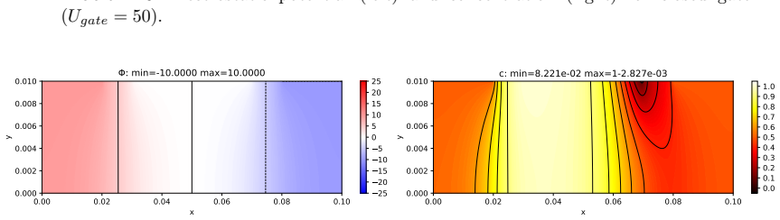
In this paper, we consider an unipolar degenerated drift-diffusion system where the relation between the concentration of the charged species $c$ and the chemical potential $h$ is $h(c)=\log \frac{c}{1-c}$. We design four different finite volume schemes based on four different formulations of the fluxes. We provide a stability analysis and existence results for the four schemes. The convergence proof with respect to the discretization parameters is established for two of them. Numerical experiments illustrate the behaviour of the different schemes.
Editorial analysis
A structured set of objections, weighed in public.
Referee Report
Summary. The paper considers the unipolar degenerated drift-diffusion system with the relation h(c) = log(c/(1-c)). It constructs four finite-volume schemes from distinct flux formulations, establishes stability and existence results for all four schemes, proves convergence with respect to discretization parameters for two of them, and presents numerical experiments comparing their behavior.
Significance. If the stability, existence, and convergence claims hold, the manuscript supplies a systematic comparison of flux formulations for a degenerate parabolic system arising in semiconductor or biological modeling. The convergence proofs for two schemes constitute a concrete contribution that can guide scheme selection; the numerical experiments provide practical illustration of the theoretical distinctions.
minor comments (2)
- The abstract states that convergence is proved for two schemes but does not identify which two or the precise sense of convergence (e.g., strong L^1 or weak-*); adding this information would improve readability.
- Notation for the admissible meshes and the discrete gradient operators should be introduced once in a dedicated preliminary section rather than repeated across scheme definitions.
Simulated Author's Rebuttal
We thank the referee for the positive assessment of the manuscript, the clear summary of its contributions, and the recommendation for minor revision. No specific major comments were listed in the report, so there are no individual points requiring point-by-point response or manuscript changes.
Circularity Check
No significant circularity; derivation is self-contained
full rationale
The paper constructs four finite volume schemes from explicit flux formulations for the given degenerate drift-diffusion model with h(c) = log(c/(1-c)). Stability, existence, and convergence results follow from direct a-priori estimates, positivity preservation, and compactness arguments on admissible meshes. No load-bearing step reduces by definition to its inputs, no fitted parameters are relabeled as predictions, and no uniqueness or ansatz is imported via self-citation chains. The modeling premise (well-posedness of the continuous system) is an external assumption standard to the field and does not create internal circularity.
Axiom & Free-Parameter Ledger
axioms (2)
- domain assumption The continuous unipolar degenerated drift-diffusion system admits solutions satisfying 0 < c < 1
- standard math Meshes are admissible in the sense required by standard finite-volume convergence theory
Reference graph
Works this paper leans on
-
[1]
A. Ait Hammou Oulhaj, C. Cancès, and C. Chainais-Hillairet. Numerical analysis of a nonlinearly stable and positive Control Volume Finite Element scheme for Richards equation with anisotropy. ESAIM: Mathematical Modelling and Numerical Analysis, 52(4):1532–1567, 2018
work page 2018
-
[2]
B. Andreianov, C. Cancès, and A. Moussa. A nonlinear time compactness result and applications to discretization of degenerate parabolic–elliptic PDEs.J. Funct. Anal., 273(12):3633–3670, 2017
work page 2017
-
[3]
M. Bessemoulin-Chatard. A finite volume scheme for convection-diffusion equations with nonlinear diffusion derived from the Scharfetter-Gummel scheme.Numer. Math., 121(4):637–670, 2012
work page 2012
-
[4]
M. Bessemoulin-Chatard, C. Chainais-Hillairet, and F. Filbet. On discrete functional inequalities for some finite volume schemes. IMA J. Numer. Anal., 35:1125–1149, 2015
work page 2015
-
[5]
J. Bezanson, Al. Edelman, S. Karpinski, and Viral B Shah. Julia: A fresh approach to numerical computing.SIAM review, 59(1):65–98, 2017
work page 2017
- [6]
-
[7]
K. Brenner, C. Cancès, and D. Hilhorst. Finite volume approximation for an immiscible two-phase flow in porous media with discontinuous capillary pressure.Comput. Geosci., 17(3):573–597, 2013
work page 2013
-
[8]
F. Brochard, J. Jouffroy, and P. Levinson. Polymer-polymer diffusion in melts.Macromolecules, 16(10):1638–1641, 1983
work page 1983
-
[9]
C. Cancès. Energy stable numerical methods for porous media flow type problems. Oil & Gas Science and Technology-Rev.IFPEN, 73:1–18, 2018
work page 2018
- [10]
-
[11]
Special issue on ”Advanced numerical methods: recent developments, analysis and application”
-
[12]
C. Cancès and C. Guichard. Convergence of a nonlinear entropy diminishing Control Volume Finite Element scheme for solving anisotropic degenerate parabolic equations.Math. Comp., 85(298):549–580, 2016
work page 2016
-
[13]
C. Cancès and C. Guichard. Numerical analysis of a robust free energy diminishing finite volume scheme for parabolic equations with gradient structure.Found. Comput. Math., 17(6):1525–1584, 2017
work page 2017
- [14]
-
[15]
C. Chainais-Hillairet, J.-G. Liu, and Y.-J. Peng. Finite volume scheme for multi-dimensional drift-diffusion equations and convergence analysis.ESAIM: M2AN, 37(2):319–338, 2003
work page 2003
-
[16]
R.Coehoorn, W.F.Pasveer, P.A.Bobbert, andM.A.J.Michels.Charge-carrierconcentrationdependenceofthehopping mobility in organic materials with gaussian disorder.Physical Review B, 72(15):155206, 2005
work page 2005
-
[17]
Y. Coudière, J.-P. Vila, and P. Villedieu. Convergence rate of a finite volume scheme for a two dimensional convection- diffusion problem.ESAIM Mathematical Modelling and Numerical Analysis, 33:493–516, 1999
work page 1999
-
[18]
Deimling.Nonlinear functional analysis
K. Deimling.Nonlinear functional analysis. Springer-Verlag, Berlin, 1985
work page 1985
- [19]
- [20]
-
[21]
J. Droniou. Finite volume schemes for diffusion equations: introduction to and review of modern methods.Math. Models Methods Appl. Sci., 24(8):1575–1620, 2014
work page 2014
-
[22]
J. Droniou and R. Eymard. The asymmetric gradient discretisation method. In C. Cancès and P. Omnes, editors,Finite volumes for complex applications VIII - methods and theoretical aspects, volume 199 ofSpringer Proc. Math. Stat., pages 311–319, Cham, 2017. Springer
work page 2017
-
[23]
J. Droniou, R. Eymard, T. Gallouët, C. Guichard, and R. Herbin.The Gradient Discretisation Method, volume 42 of Mathématiques et Applications. Springer International Publishing, 2018
work page 2018
-
[24]
R. Eymard and T. Gallouët. H-convergence and numerical schemes for elliptic problems.SIAM J. Numer. Anal., 41(2):539–562, 2003
work page 2003
- [25]
- [26]
-
[27]
P. Farrell, T. Koprucki, and J. Fuhrmann. Computational and analytical comparison of flux discretizations for the semiconductor device equations beyond Boltzmann statistics.J. Comput. Phys., 346:497–513, 2017
work page 2017
- [28]
- [29]
-
[30]
J. Fuhrmann. UnipolarDriftDiffusion.jl - Numerical examples for finite volume schemes for unipolar drift-diffusion problems, 2019. URL:https://github.com/j-fu/UnipolarDriftDiffusion.jl, DOI:10.5281/zenodo.3351467
-
[31]
J. Fuhrmann. VoronoiFVM.jl - Solver for coupled nonlinear partial differential equations based on the Voronoi finite volume method, 2019. URL:https://github.com/j-fu/VoronoiFVM.jl, DOI:10.5281/zenodo.3351449
-
[32]
J. Fuhrmann and C. Guhlke. A finite volume scheme for Nernst-Planck-Poisson systems with ion size and solvation effects. In C. Cancès & P. Omnes, editor,Finite Volumes for Complex Applications VIII - Hyperbolic, Elliptic and Parabolic Problems, volume 200 ofSpringer Proceedings in Mathematics & Statistics, pages 497–505, Lille, France,
-
[33]
Springer International Publishing
- [34]
-
[35]
N. Gavish and A. Yochelis. Theory of phase separation and polarization for pure ionic liquids.The journal of physical chemistry letters, 7(7):1121–1126, 2016
work page 2016
-
[36]
A. Glitzky and J. A. Griepentrog. Discrete Sobolev-Poincaré inequalities for Voronoi finite volume approximations. SIAM J. Numer. Anal., 48:372–391, 2010
work page 2010
-
[37]
Hackbusch.Elliptic Differential Equations: Theory and Numerical Treatment
W. Hackbusch.Elliptic Differential Equations: Theory and Numerical Treatment. Springer Series in Computational Mathematics 18. Springer-Verlag Berlin Heidelberg, 2nd edition, 2017
work page 2017
-
[38]
R. Herbin. An error estimate for a finite volume scheme for a diffusion–convection problem on a triangular mesh. Numer. Methods Partial Differential Equations, 11(2):165–173, 1995
work page 1995
-
[39]
T. Koprucki and K. Gärtner. Discretization scheme for drift-diffusion equations with strong diffusion enhancement. Optical and Quantum Electronics, 45(7):791–796, 2013
work page 2013
-
[40]
J. Leray and J. Schauder. Topologie et équations fonctionnelles.Ann. Sci. École Norm. Sup. (3), 51:45–78, 1934
work page 1934
-
[41]
G. Paasch and S. Scheinert. Charge carrier density of organics with gaussian density of states: analytical approximation for the Gauss–Fermi integral.Journal of Applied Physics, 107(10):104501, 2010
work page 2010
-
[42]
Forward-Mode Automatic Differentiation in Julia
J. Revels, M. Lubin, and T. Papamarkou. Forward-mode automatic differentiation in julia.arXiv:1607.07892 [cs.MS], 2016
work page internal anchor Pith review Pith/arXiv arXiv 2016
-
[43]
D. L. Scharfetter and H. K. Gummel. Large-signal analysis of a silicon read diode oscillator.Electron Devices, IEEE Transactions on, 16(1):64–77, 1969
work page 1969
-
[44]
Selberherr.Analysis and simulation of semiconductor devices
S. Selberherr.Analysis and simulation of semiconductor devices. Springer, 2012
work page 2012
- [45]
- [46]
-
[47]
Z. Yu and R. Dutton. SEDAN III. www-tcad.stanford.edu/tcad/programs/sedan3.html, 1998. Clément Cancès ( clement.cances@inria.fr): Inria, Univ. Lille, CNRS, UMR 8524 - Laboratoire Paul Painlevé, F-59000 Lille Claire Chainais-Hillairet ( claire.chanais@univ-lille.fr): Univ. Lille, CNRS, UMR 8524, Inria - Labo- ratoire Paul Painlevé, F-59000 Lille Jürgen Fuh...
work page 1998
discussion (0)
Sign in with ORCID, Apple, or X to comment. Anyone can read and Pith papers without signing in.