Slope-Dependent Rendering of Parallel Coordinates to Reduce Density Distortion and Ghost Clusters

Daniel A. Keim; David Pomerenke; Frederik L. Dennig; Johannes Fuchs; Michael Blumenschein

REVIEW 3 major objections 5 minor 21 references

Slope-Dependent Rendering of Parallel Coordinates to Reduce Density Distortion and Ghost Clusters

T0 review · 3 major / 5 minor · reviewed 2026-08-14 · deepseek-v4-flash

Challenge this review Re-run · record.json Download PDF Read on arXiv ↗ Review JSON

Pith's one-line read The paper argues that the slope of polyline segments in parallel coordinates biases perceived cluster density, and that drawing each segment with width $\omega = h\cos(\alpha)$ equalizes ink per data record and reduces ghost clusters.

desk verdict The geometry is right and the rendering fix is sensible, but the perceptual benefit is asserted from example images, not measured; the authors openly defer a user study. read the letter →

arxiv 1908.00500 v2 pith:FGML375Z submitted 2019-08-01 cs.GR

David Pomerenke , Frederik L. Dennig , Daniel A. Keim , Johannes Fuchs , Michael Blumenschein This is my paper · ORCID

classification cs.GR

keywords parallelcoordinatesdensitydistortionghostclustersslope-dependentrenderinglinewidthpolylinevisualperceptiondata-inkratio

verification ladder T0 review T1 audit T2 compute T3 formal

The pith

A machine-rendered reading of the paper's core claim, the machinery that carries it, and where it could break.

The reading

Parallel coordinates draw every data record as a polyline, but a segment's visual weight depends on its slope: diagonal segments are longer, cover more pixels, and lie closer to neighboring segments than horizontal segments describing the same data. The paper formalizes this as a slope-dependent distortion of cluster density and shows that it can manufacture ghost clusters in uniformly random data. To fix it, the paper proposes giving each segment width $\omega = h\cos(\alpha)$, so all segments have the same surface area regardless of slope, with a parameter $P$ in $\omega = h\cos^P(\alpha)$ to tune between no correction and over-correction. The rendering is linear-time, depends on one parameter, and composes with most existing parallel-coordinate variants. If the claim holds, cluster prominence in parallel coordinates would reflect data structure rather than accidental angle, and noise would stop masquerading as clusters.

What carries the argument

The load-bearing object is a polyline segment reinterpreted as a parallelogram of constant area. Requiring the area $A$ to be the same for every segment fixes the width as $\omega = A/l = h\cos(\alpha)$, because the segment length is $l=\Delta W/\cos(\alpha)$ and $A=\Delta W\,h$. The generalized law $\omega = h\cos^P(\alpha)$ is the single tuning parameter of the method: $P$ decides whether the correction is absent, full, or over-corrected. This identity carries the argument because it turns the perceptual complaint (steep segments occupy more pixels and sit closer together) into one per-segment quantity, the stroke width, which can be computed on the fly for any polyline and layered onto existing parallel-coordinate renderings.

What would settle it

A controlled experiment could settle the claim: show participants panels containing one horizontal and one diagonal cluster with identical data size, rendered at $P=0$, $P=1$, and $P=2$, and ask which cluster appears more prominent. If at $P=1$ users still systematically rate the diagonal cluster as stronger, or still report ghost clusters in uniformly random data, then equalizing rendered line area is not sufficient to correct the perceptual distortion.

Watch

Extended reading notes

Core claim

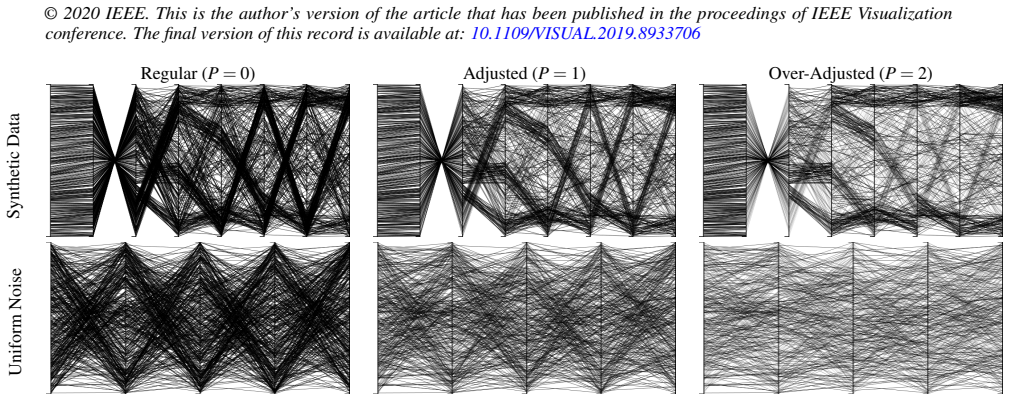
The central claim is that classical parallel-coordinate rendering distorts cluster density because every geometric property of a segment depends on its angle $\alpha$: length $l=\Delta W\cos^{-1}(\alpha)$, line height $h = w\cos^{-1}(\alpha)$, area, and pixel count all grow steeply with slope, while the orthogonal distance $d_\perp$ between neighboring segments shrinks as $\cos(\alpha)$. Treating a segment as a parallelogram with constant area $A = l\cdot\omega = \Delta W\,h$ yields the slope-dependent width $\omega = h\cos(\alpha)$; generalizing to $\omega = h\cos^P(\alpha)$ interpolates from classical rendering ($P=0$) through equal-area rendering ($P=1$) to over-adjustment ($P=2$) that also compensates reduced inter-line spacing. The paper argues that this width law removes the extra emphasis diagonal clusters receive and reduces the visibility of ghost clusters in uniform noise, and that it can be computed in linear time as a per-segment stroke width.

Load-bearing premise

The load-bearing premise is that Gestalt proximity — rendered line density and spacing — is the dominant cue for cluster perception in parallel coordinates, so equalizing those quantities across slopes will make perception match the data; the paper asserts this from the Gestalt literature but presents no user study to confirm it.

Editorial extensions

If this is right

With $P=1$, diagonal and horizontal clusters receive equal line area, so cluster prominence in a plot reflects the data rather than the segment angle.
Because the correction is only a per-segment stroke-width change, rendering stays linear in the number of segments and adds no asymptotic cost.
Uniform random noise is less likely to produce perceptible ghost clusters, since the false density that made a few steep parallel lines cohere is removed.
The method composes with axes reordering, dimension reduction, and density-based or bundling variants of parallel coordinates, extending clutter reduction rather than competing with it.
Choosing $P>1$ over-corrects: it further suppresses ghost clusters and compensates the reduced inter-line spacing of steep segments, but begins to over-emphasize horizontal clusters, so $P\approx 2$ is suggested as an upper bound.

Reading between the lines

Editorial extensions of the paper, not claims the author makes directly.

Beyond the paper: the same parallelogram-area principle could apply to other line-based charts where segment length varies with orientation, such as slope charts, with stroke width inversely proportional to rendered length to enforce equal ink per record.
Beyond the paper: since parameter selection is left manual, a natural data-driven next step is to measure the distribution of segment angles and overplotting in screen space and choose $P$ so that the per-angle pixel histogram becomes flat.
Beyond the paper: because the paper reports qualitative testing but no user study, a testable prediction implied by its argument is that users' cluster-counting accuracy on identical datasets improves under $P=1$ relative to classical rendering.

Share X Bluesky LinkedIn Reddit HN

Signed reviews

No signed human review yet.

Editorial analysis

A structured set of objections, weighed in public.

Desk editor's note, referee report, and a circularity audit.

Desk Editor's Note

read the letter

The geometric core of this paper is genuinely sound, and the contribution is real, if modest. The authors are the first to explicitly formalize the slope-dependent density distortion in parallel coordinates: line length and area scale as cos^-1(alpha), orthogonal distance as cos(alpha), and clusters at steep angles get both more ink and less separation. The proposed fix, rendering with width omega = h * cos^P(alpha), is a natural and clean response. With P=1 every segment has the same surface area, the derivation is straightforward, and the method runs in linear time and composes with most other PCP techniques. They also ship code and data, which is more than many vis papers do. I credit the open materials and the honest accounting of what the geometry does and does not fix.

The soft spot is exactly where the stress-test lands. The paper's central claim is perceptual: slope-dependent rendering reduces ghost clusters and balances cluster prominence. What is actually shown is that the geometric quantities are equalized, plus side-by-side images. Section 5 explicitly says a quantitative user study is future work. That is a real omission for a paper whose selling point is perception, not just pixel area. The Gestalt proximity argument in Section 3.3 is plausible but unexamined; if other cues—continuity, crossings, color, transparency—carry more weight, the benefit could shrink. Also, the paper itself admits that P=1 does not correct the distance compression d_perp = d_h * cos(alpha); only P>1 reduces it, at the cost of over-emphasizing horizontal lines. So the abstract's phrase "avoids density distortions" is too strong for what the recommended setting delivers; "reduces" would be honest. These are proportionate criticisms, not fatal ones. The authors are transparent about the limitation, and the formal contribution stands independently of the missing user study.

The citation pattern looks normal and the related work is adequate, with Zhou et al.'s splatting correctly identified as closest. No circular reasoning; the free parameter P is an explicit user choice, not fitted to force an outcome.

Who is this for? Anyone working on parallel coordinates, clutter reduction, or perception-oriented rendering in information visualization. It is a short, readable paper with a useful observation and a practical tweak. It deserves a serious referee, and a fair review would ask for a user study or a more carefully scoped claim, not reject it outright. I would bring it to a reading group and would cite it if I were writing on PCP rendering.

Referee Report

3 major / 5 minor

Summary. The paper addresses a geometric distortion inherent to parallel coordinates: polyline segments of different slopes are rendered with different pixel areas and different orthogonal distances between parallel lines, making diagonal clusters appear denser and more prominent than horizontal ones and causing ghost clusters in uniformly random data. The paper formalizes the geometry of a segment (length, height, and area as functions of the angle α), then proposes rendering each segment with an angle-dependent width ω = h·cos^P(α), where P = 0 reproduces classical rendering, P = 1 makes segment surface area constant, and P > 1 over-adjusts to partially compensate for the reduced line distance at steep slopes. The authors provide qualitative comparisons on synthetic and real data, an interactive tool, and a discussion of parameters; they explicitly defer a quantitative user study to future work.

Significance. If the perceptual premise holds, the paper makes a useful contribution: the geometric derivation is transparent, depends on no fitted parameters except the user-chosen strength P, the technique runs in linear time and composes with axes reordering, dimension reduction, and edge bundling, and the authors provide code and an online tool. The formalization of slope-dependent density distortion is itself a valuable contribution that could inform other parallel-coordinate variants. The main weakness is that the central perceptual claims are asserted rather than measured: the argument connects rendered ink density to cluster perception via the Gestalt law of proximity, but no user study or quantitative perceptual metric is reported, and Section 5 explicitly defers such an evaluation. The equal-area property alone does not establish that cluster perception improves or that ghost clusters are reduced for human observers.

major comments (3)

[Abstract and Section 4.1] The abstract's claim that the technique 'avoids density distortions of clusters' is stronger than what the manuscript establishes. Section 4.1 states that P = 1 equalizes surface area but does not correct the reduced orthogonal line distance d⊥ = dh·cos(α); only P > 1 reduces that distance further, at the cost of over-emphasizing horizontal lines. The wording should be qualified to say that the method mitigates the area component at P = 1 and can reduce, but not fully eliminate, the distance component with over-adjustment.
[Section 3.3 and Section 5] The load-bearing perceptual model is unvalidated. The paper invokes the Gestalt law of proximity to translate rendered line density and distance into perceived cluster cohesiveness, but it provides no user study, no perceptual threshold data, and no quantitative comparison of cluster-detection accuracy or perceived prominence among P = 0, P = 1, and P = 2; Section 5 defers this to future work. Because the stated contribution is to reduce density distortion and ghost clusters as perceived by users, the illustrative images in Figures 1, 4, and 5 are not sufficient evidence. The authors should either add a controlled experiment with error bars or explicitly limit the claims to the geometric properties of the rendering.
[Section 4.1] The guidance for choosing P is informal and not systematically supported. The paper recommends P = 1 for truthful representation but states that 'P ≈ 2 is an upper bound for most applications' based on 'our tests' without reporting the datasets, tasks, or metrics used; Section 5 adds that P cannot be determined automatically. Since the visual outcome changes substantially with P (as Figure 5 shows), the paper should either report a sensitivity analysis or clearly frame P as an interactive parameter whose effect is demonstrated only anecdotally.

minor comments (5)

[Section 3.1 and Section 4] The symbol h is used for two different quantities: in Section 3.1, h is the slope-dependent line height given by h = w·cos⁻¹(α), while in Section 4, h is the constant side length of the parallelogram. Reusing h this way is confusing; one of the two quantities should be renamed (for example, w_h for the height).
[Figure 4] The caption of Figure 4(d), '(d) = (c) but the data points of a ghost cluster are highlighted', is ungrammatical and unclear; it should read something like '(d) is the same plot as (c), with the polylines of one apparent ghost cluster highlighted'.
[Section 4] Equations (1) and (2) are introduced without an explicit reference in the surrounding text; the discussion in Section 4.1 would be easier to follow if the equations were cited directly when P = 0, P = 1, and P > 1 are discussed.
[Section 4.2] The final sentence about transparency states that 'Adjusting the transparency of lines based on their slopes, as opposed to the line width, is not useful' without an argument or citation. This is an unexplained design claim and should be supported or removed.
[Section 5] The OSF link in the introduction and the GitHub and tool links in Section 5 should be consolidated into a single data-availability statement, and the authors should verify that these links resolve to the stated artifacts.

Circularity Check

0 steps flagged · score 0.0 of 10

No circular reasoning: the width formula is derived from the goal of constant segment area, and no fitted parameter or self-citation chain is load-bearing.

full rationale

The paper's central derivation is self-contained and non-circular. Section 3.1 defines the geometry: h = w·cos^(-1)(α), so the segment area is A = h·ΔW. Section 4 then solves for the width that makes A constant: ω = h·cos(α), since l·ω = (ΔW/cos α)·(h·cos α) = ΔW·h. This is an exact derivation from the stated goal of equal line-segment area; no quantity is fitted to a target outcome. The generalized exponent P is a user-controlled adjustment strength, not a fitted parameter, and the paper explicitly recommends P=1 for truthful representation and notes that P>1 trades off horizontal over-emphasis. The ghost-cluster and perception claims rest on external Gestalt-proximity citations (Koffka, Ware) and on qualitative examples; Section 5 states that a quantitative user study is future work. That is an evidentiary limitation, not circularity: the perceptual benefit is asserted rather than measured, but the geometric correction itself follows from the problem formalization and is not equivalent by construction to the claimed empirical effect.

Assumptions & free parameters 1 free parameters · 3 assumptions · 0 invented entities

The central claim rests on standard Euclidean geometry (which is correctly derived) and on perceptual assumptions about how line density creates perceived clusters. The only free parameter is the user-chosen P. No new entities are introduced.

free parameters (1)

P (adjustment strength) = user-selected; recommended P=1, upper bound P approximately 2
Controls how strongly line width varies with slope. Not fitted to data; the paper says P cannot be determined automatically (Sections 4.1 and 5).

assumptions (3)

domain assumption The Gestalt law of proximity: perceived cluster cohesiveness increases with line density
Invoked in Section 3.3 to argue that density distortion translates into perceived cluster strength; no empirical test is reported.
domain assumption Visual cluster density is appropriately measured by the share of colored pixels and the orthogonal distance between polylines
Section 3.2 defines visual cluster density this way; the technique optimizes these quantities, assuming they are the correct perceptual proxies.
domain assumption Users expect a PCP to be orientation-neutral, that is, not to emphasize diagonal vs horizontal patterns by default
Stated in Section 3.3 and implicitly required for the goal of the correction to be desirable.

how reviews work

0 comments

Cite this review

Pith. "Pith review of Slope-Dependent Rendering of Parallel Coordinates to Reduce Density Distortion and Ghost Clusters." pith.science (2026). https://pith.science/paper/FGML375Z

@misc{pith2026190800500,
  author       = {Pith},
  title        = {Pith review of: Slope-Dependent Rendering of Parallel Coordinates to Reduce Density Distortion and Ghost Clusters},
  year         = {2026},
  howpublished = {\url{https://pith.science/paper/FGML375Z}},
  note         = {Machine review of arXiv:1908.00500}
}

read the original abstract

Parallel coordinates are a popular technique to visualize multi-dimensional data. However, they face a significant problem influencing the perception and interpretation of patterns. The distance between two parallel lines differs based on their slope. Vertical lines are rendered longer and closer to each other than horizontal lines. This problem is inherent in the technique and has two main consequences: (1) clusters which have a steep slope between two axes are visually more prominent than horizontal clusters. (2) Noise and clutter can be perceived as clusters, as a few parallel vertical lines visually emerge as a ghost cluster. Our paper makes two contributions: First, we formalize the problem and show its impact. Second, we present a novel technique to reduce the effects by rendering the polylines of the parallel coordinates based on their slope: horizontal lines are rendered with the default width, lines with a steep slope with a thinner line. Our technique avoids density distortions of clusters, can be computed in linear time, and can be added on top of most parallel coordinate variations. To demonstrate the usefulness, we show examples and compare them to the classical rendering.

Figures

Figures reproduced from arXiv: 1908.00500 by the authors.

**Figure 1.** Comparison of regular parallel coordinates with our slope-dependent polyline rendering. Parallel coordinates face two problems, which are inherent in the technique: (a) depicts three clusters of the same diameter and size across all dimensions. Diagonal changes of the clusters are visually more prominent, as diagonal lines are rendered more closely. (c) shows 200 data points of uniform random clutter/noise in all di… view at source ↗

**Figure 3.** Effect of angle α on PCP lines. (1) Diagonal lines have a higher line surface area (= more pixels) compared to horizontal lines. (2) Diagonal lines have a smaller distance between lines. 2 [PITH_FULL_IMAGE:figures/full_fig_p002_3.png] view at source ↗

**Figure 4.** Ghost clusters in uniformly distributed random data points. The number n of polylines is increased from (a) to (c). (d) = (c) but the data points of a ghost cluster are highlighted to demonstrate that they are indeed uniformly distributed even though (c) indicates otherwise. and therefore a more prominent line. The emphasis translates from lines to clusters, so that diagonal clusters are more noticeable than horizon… view at source ↗

Figures from the paper (1 more)

**Figure 5.** Figure 5: Effect of parameter P on pattern visualization in synthetic data with uniformly distributed background noise, and in uniformly distributed random data only. Regular rendering (P = 0) significantly over-emphasizes diagonal clusters and causes the occurrence of ghost clu…

Discussion (0). Continue with ORCID to comment.

Reference graph

Works this paper leans on

21 extracted references · 15 canonical work pages

[1]

Alsakran, Y

J. Alsakran, Y . Zhao, and X. Zhao. Tile-based parallel coordinates and its application in ﬁnancial visualization. In Visualization and Data Analysis, 2010. doi: 10.1117/12.838819

work page doi:10.1117/12.838819 2010
[2]

Andrienko and N

G. Andrienko and N. Andrienko. Constructing parallel coordinates plot for problem solving. In 1st International Symposium on Smart Graphics, pp. 9–14, 2001

work page 2001
[3]

Bachthaler and D

S. Bachthaler and D. Weiskopf. Continuous scatterplots. IEEE Trans- actions on Visualization and Computer Graphics, 14(6):1428–1435,

work page
[4]

Behrisch, M

M. Behrisch, M. Blumenschein, N. W. Kim, L. Shao, M. El-Assady, J. Fuchs, D. Seebacher, A. Diehl, U. Brandes, H. Pﬁster, T. Schreck, D. Weiskopf, and D. A. Keim. Quality metrics for information visu- alization. Computer Graphics Forum, 37(3):625–662, 2018. doi: 10. 1111/cgf.13446

work page 2018
[5]

Dasgupta and R

A. Dasgupta and R. Kosara. Pargnostics: Screen-space metrics for parallel coordinates. IEEE Transactions on Visualization and Computer Graphics, 16(6):1017–1026, 2010. doi: 10.1109/TVCG.2010.184

doi:10.1109/tvcg.2010.184 2010
[6]

G. P. Ellis and A. J. Dix. A taxonomy of clutter reduction for informa- tion visualisation. IEEE Transactions on Visualization and Computer Graphics, 13(6):1216–1223, 2007. doi: 10.1109/TVCG.2007.70535

arXiv 2007
[7]

Y . Fua, M. O. Ward, and E. A. Rundensteiner. Hierarchical parallel coordinates for exploration of large datasets. In IEEE Conference on Visualization, pp. 43–50, 1999. doi: 10.1109/VISUAL.1999.809866

work page arXiv 1999
[8]

Heinrich, Y

J. Heinrich, Y . Luo, A. E. Kirkpatrick, and D. Weiskopf. Evaluation of a bundling technique for parallel coordinates. In Proceedings of the International Conference on Computer Graphics Theory and Ap- plications and International Conference on Information Visualization Theory and Applications, pp. 594–602, 2012

work page 2012

Show all 21 references

[9]

Heinrich and D

J. Heinrich and D. Weiskopf. Continuous parallel coordinates. IEEE Transactions on Visualization and Computer Graphics, 15(6):1531– 1538, 2009. doi: 10.1109/TVCG.2009.131

2009 doi
[10]

Heinrich and D

J. Heinrich and D. Weiskopf. State of the art of parallel coordinates. In Eurographics 2013 - State of the Art Reports, , pp. 95–116. The Eurographics Association, 2013. doi: 10.2312/conf/EG2013/stars/095 -116

2013 doi
[11]

Inselberg

A. Inselberg. The plane with parallel coordinates.The Visual Computer, 1(2):69–91, 1985. doi: 10.1007/BF01898350

1985 doi
[12]

Johansson, P

J. Johansson, P. Ljung, M. Jern, and M. D. Cooper. Revealing structure within clustered parallel coordinates displays. In IEEE Symposium on Information Visualization, pp. 125–132, 2005. doi: 10.1109/INFVIS. 2005.1532138

2005
[13]

K. Koffka. Principles of Gestalt psychology. Mimesis International, September 2014

2014
[14]

Palmas, M

G. Palmas, M. Bachynskyi, A. Oulasvirta, H. Seidel, and T. Weinkauf. An edge-bundling layout for interactive parallel coordinates. In IEEE Paciﬁc Visualization Symposium , pp. 57–64, 2014. doi: 10.1109/ PaciﬁcVis.2014.40

2014
[15]

Siirtola, T

H. Siirtola, T. Laivo, T. Heimonen, and K. R¨aih¨a. Visual perception of parallel coordinate visualizations. In 13th International Conference on Information Visualisation, pp. 3–9, 2009. doi: 10.1109/IV.2009.25

2009 doi
[16]

Siirtola and K

H. Siirtola and K. R¨aih¨a. Interacting with parallel coordinates. Inter- acting with Computers, 18(6):1278–1309, 2006. doi: 10.1016/j.intcom .2006.03.006

2006 doi
[17]

Stockinger, K

K. Stockinger, K. Wu, S. Campbell, S. Lau, M. Fisk, E. M. Gavrilov, A. Kent, C. E. Davis, R. D. Olinger, R. J. Young, J. Prewett, P. M. We- ber, T. P. Caudell, E. W. Bethel, and S. Smith. Network trafﬁc analysis with query driven visualization SC 2005 HPC analytics results. In...

2005 doi
[18]

E. R. Tufte. The Visual Display of Quantitative Information. Graphics Press, Cheshire, CT, USA, 2nd ed., 2001

2001
[19]

C. Ware. Information visualization: perception for design . Morgan Kaufmann, 3rd ed., May 2012

2012
[20]

H. Zhou, W. Cui, H. Qu, Y . Wu, X. Yuan, and W. Zhuo. Splatting the lines in parallel coordinates. Computer Graphics Forum, 28(3):759– 766, 2009. doi: 10.1111/j.1467-8659.2009.01476.x 5

2009
[2008]

doi: 10.1109/TVCG.2008.119

2008 doi

Pith tools

Reviewed August 14, 2026 · model on record in the stance chip above.

[1] [1]

Alsakran, Y

J. Alsakran, Y . Zhao, and X. Zhao. Tile-based parallel coordinates and its application in ﬁnancial visualization. In Visualization and Data Analysis, 2010. doi: 10.1117/12.838819

work page doi:10.1117/12.838819 2010

[2] [2]

Andrienko and N

G. Andrienko and N. Andrienko. Constructing parallel coordinates plot for problem solving. In 1st International Symposium on Smart Graphics, pp. 9–14, 2001

work page 2001

[3] [3]

Bachthaler and D

S. Bachthaler and D. Weiskopf. Continuous scatterplots. IEEE Trans- actions on Visualization and Computer Graphics, 14(6):1428–1435,

work page

[4] [4]

Behrisch, M

M. Behrisch, M. Blumenschein, N. W. Kim, L. Shao, M. El-Assady, J. Fuchs, D. Seebacher, A. Diehl, U. Brandes, H. Pﬁster, T. Schreck, D. Weiskopf, and D. A. Keim. Quality metrics for information visu- alization. Computer Graphics Forum, 37(3):625–662, 2018. doi: 10. 1111/cgf.13446

work page 2018

[5] [5]

Dasgupta and R

A. Dasgupta and R. Kosara. Pargnostics: Screen-space metrics for parallel coordinates. IEEE Transactions on Visualization and Computer Graphics, 16(6):1017–1026, 2010. doi: 10.1109/TVCG.2010.184

doi:10.1109/tvcg.2010.184 2010

[6] [6]

G. P. Ellis and A. J. Dix. A taxonomy of clutter reduction for informa- tion visualisation. IEEE Transactions on Visualization and Computer Graphics, 13(6):1216–1223, 2007. doi: 10.1109/TVCG.2007.70535

arXiv 2007

[7] [7]

Y . Fua, M. O. Ward, and E. A. Rundensteiner. Hierarchical parallel coordinates for exploration of large datasets. In IEEE Conference on Visualization, pp. 43–50, 1999. doi: 10.1109/VISUAL.1999.809866

work page arXiv 1999

[8] [8]

Heinrich, Y

J. Heinrich, Y . Luo, A. E. Kirkpatrick, and D. Weiskopf. Evaluation of a bundling technique for parallel coordinates. In Proceedings of the International Conference on Computer Graphics Theory and Ap- plications and International Conference on Information Visualization Theory and Applications, pp. 594–602, 2012

work page 2012