REVIEW 4 minor 34 references
Deterministic and randomized motions in single-well potentials
T0 review · 0 major / 4 minor · reviewed 2026-08-14 · deepseek-v4-flash
Pith's one-line read This paper establishes that random hard velocity reversals leave the asymptotic position and velocity statistics of a particle in a single-well potential exactly equal to the deterministic orbit's statistics, regardless of the…
desk verdict Correct, modest extension of the authors' earlier work; the main claim survives the flagged 2D-orbit objection, but the abstract overstates heavy-tailed convergence. read the letter →
The pith
A machine-rendered reading of the paper's core claim, the machinery that carries it, and where it could break.
The reading
What carries the argument
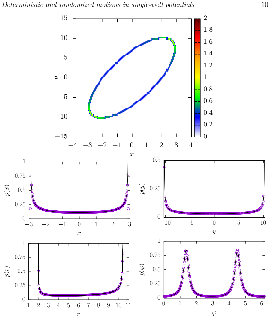
The load-bearing object is the constant-energy orbit and the period T of the deterministic motion. The density construction starts from the time-averaging relation p(x)dx = (2/T)dx/v, which says that the probability of finding the particle near x is proportional to the time it spends there, and the energy relation E = mv²/2 + κ|x|^n supplies v as a function of x. A hard velocity reversal maps the state (x,v) to (x,-v), preserving both position and total energy, so the randomized process never leaves the same energy surface and its stationary measure must be the same invariant measure as the deterministic flow; combining the period with the energy relation gives the explicit formulas. In two dimensions, the same logic is carried by the effective radial potential U_eff(r) = L²/(2mr²) + κr^n and the radial energy relation (m/2)ṙ² = E - U_eff(r), which yields p(r) ∝ 1/√(E - U_eff(r)).
What would settle it
Run the randomized one-dimensional dynamics to a very large observation time with a fixed initial condition and a waiting-time distribution with finite mean, such as an exponential distribution, and check whether the measured p(x) and p(v) converge to Eqs. (5) and (6) with the prescribed normalization; a persistent mismatch would falsify the central claim. For heavy-tailed waiting times with α<1, simulate to times far beyond t=1000 and test whether the remnant deterministic peak decays to the smooth density, and in 2D with n=4 compare the long-run normalized p(r) histogram against Eq. (D.12) for several initial conditions.
Extended reading notes
Core claim
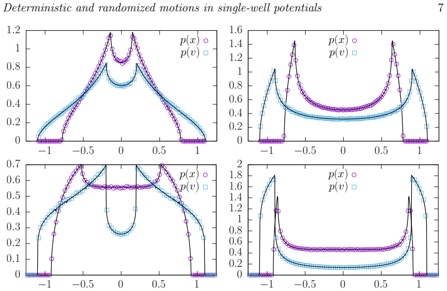
For a particle of mass m in a one-dimensional potential V(x)=κ|x|^n with a fixed initial condition and total energy E, the long-observation probability density of position is p(x) = (2/T)[(2/m)(E - κ|x|^n)]^{-1/2} and the density of velocity is p(v) = (2m/(Tκn))[(1/κ)(E - mv²/2)]^{1/n-1}, where T is the deterministic period. Interrupting the deterministic motion by hard velocity reversals, v(t_i)→-v(t_i), at random times drawn from any one-sided waiting-time distribution p(τ) produces, asymptotically, exactly these same densities, so the asymptotic statistics of the randomized process coincide with those of the deterministic trajectory and are independent of p(τ). In two dimensions with a central potential V(r)=κr^n, the same asymptotic insensitivity holds for marginal densities; the radial density is p(r) ∝ 1/√(E - L²/(2mr²) - κr^n), where L is the conserved angular momentum and the effective potential U_eff(r)=L²/(2mr²)+κr^n bounds the radial motion. The randomization thus makes ensemble averages interchangeable with time averages along a single constant-energy trajectory, while randomization of initial conditions breaks this equivalence and yields a mixture of fixed-energy densities.
Load-bearing premise
The broadest load-bearing premise is that in the long-time limit the randomized trajectory with velocity reversals explores the entire constant-energy, and in 2D constant-angular-momentum, available region in the same statistical proportions as the deterministic orbit, so that time and ensemble averages coincide; for 2D non-closed orbits and for reversal times with diverging mean this is verified numerically at finite time rather than proven.
Editorial extensions
If this is right
- For a fixed initial condition, long time averages and ensemble averages over the randomized process give identical asymptotic densities, so simulations with velocity reversals can be used interchangeably with long deterministic trajectories to estimate p(x) and p(v).
- The exact waiting-time distribution p(τ) only shapes transients; all choices with finite mean lead to the same stationary densities, so measured asymptotic statistics cannot be used to infer the reversal-time statistics.
- Randomizing initial conditions changes the story: the resulting densities are mixtures of the fixed-energy densities and can be far from the arcsine-like shapes, with closed-form hypergeometric expressions for uniform energy distributions.
- In two dimensions, exact marginal densities are available for the harmonic well (n=2), and the radial density p(r) ∝ [E - L²/(2mr²) - κr^n]^{-1/2} holds generally, with hard velocity reversals not altering these asymptotics.
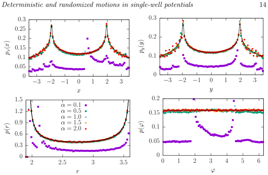
- For heavy-tailed waiting times with diverging mean (α<1), the stationary limit is approached only slowly; at finite observation time a peak corresponding to the initial condition remains, so the insensitivity is an asymptotic rather than a finite-time statement.
Reading between the lines
- The same asymptotic equivalence may hold for any bounded conservative one-dimensional system whose deterministic orbit is a single closed loop, because the construction uses only the period and the constant-energy curve, not the specific monomial form of the potential.
- The paper's two-dimensional result for non-closed orbits implicitly assumes that the quasi-periodic trajectory samples the accessible annulus densely enough for time averages to converge to the steady densities; a rigorous ergodic statement, or a counterexample with a resonant orbit, would sharpen the claim.
- A natural extension is to replace hard reversals by other energy-preserving random kicks, such as rotating the velocity vector in 2D; if the invariant measure on the energy surface is unique, the same asymptotic densities should appear.
- The slow convergence observed for reversal-time distributions with diverging mean suggests that in practical finite-time experiments the reversal-time distribution still matters; a quantitative estimate of the decay rate of the initial-condition peak would be useful for applications to Lévy-walk-type models.
Signed reviews
Editorial analysis
A structured set of objections, weighed in public.
Referee Report
Summary. This paper studies deterministic Newtonian motion in single-well potentials of the form V(x)=κ|x|n in one and two dimensions and compares the long-time statistical properties of the deterministic orbit with those of a randomized process in which the velocity is reversed at random time instants (hard velocity reversals). The authors derive exact expressions for the stationary position and velocity densities in 1D for arbitrary n (Eqs. (5)-(6) and Appendix A), and an exact formula for the radial density in 2D via the effective potential (Eq. (D.12)). They present Monte Carlo simulations showing that the asymptotic densities are insensitive to the distribution of waiting times between reversals, both in 1D and for the marginal densities in 2D, and that randomization of initial conditions instead leads to modified densities. The paper also discusses transient effects for heavy-tailed waiting-time distributions.
Significance. The main contribution is the explicit confirmation that energy-conserving velocity reversals at random times do not alter the long-time distribution of a conservative system in a single-well potential, generalizing earlier results of Dybiec et al. [5] to arbitrary exponent n and to the 2D radial density. The derivations are elementary and transparent, and the numerical simulations agree with the analytical predictions in the parameter regimes studied. The paper provides a clean example of the equivalence of time and ensemble averaging under a specific randomization, and it offers useful formulas for researchers working on Lévy-walk-type models in external potentials. The novelty is moderate, but the results are solid and clearly presented.
minor comments (4)
- [Appendix B, Eq. (B.1)] The formula for \tilde{p}(E,v) contains x^2 in several places where v^2 must appear, e.g., "1 - m x^2/(2E)" and "2E/(m x^2)", while the stated condition of validity is E - m v^2/2 > 0. This inconsistency makes the printed expression unusable; please correct the variable name throughout the equation.
- [Section 3.2.1, paragraph on Fig. 5] The text reads "Distances from the origin to apocenters (rmin) and pericenters (rmax)" and later "the apocenter (rmin) and the pericenter (rmin)"; the labels are switched. The apocenter is the largest radius (rmax) and the pericenter is the smallest radius (rmin).
- [Section 3.2.2, Figs. 6-7] The extrapolation to t→∞ for heavy-tailed waiting times with α<1 is based on simulations at t=1000 that still show a residual deterministic peak. A brief explanation of why the peak is expected to vanish (e.g., the probability of no reversal decays as t^{-α}) would make the asymptotic claim more persuasive.
- [Abstract and Section 3.2.2] The abstract states a general insensitivity of probability distributions to velocity reversals in 2D. While the radial density p(r) follows exactly from the 1D reduction in Appendix D, the corresponding statement for px(x), py(y), and p(ϕ) is supported in the manuscript only by finite-time numerics for n≠2. A sentence clarifying which 2D results are proven and which are numerical would bring the wording in line with the evidence presented.
Circularity Check
No significant circularity: stationary densities follow from mechanics and the randomized equivalence is supported by independent, parameter-free simulation.
full rationale
The paper's analytical derivation chain is self-contained. In Appendix A, the 1D stationary densities p(x) and p(v), Eqs. (5)-(6), are obtained from the definition of occupation time, p(x)dx=(2/T)dx/v (Eq. A.1), the period T (Eq. A.2), and energy conservation v = sqrt(2[E-kappa|x|^n]/m) (Eqs. A.3-A.4); p(v) then follows by a change of variables (Eqs. A.6-A.9). No parameter is fitted to force agreement with the randomized simulations. The 2D radial density p(r) proportional to 1/rdot, Eq. (D.12), is likewise derived from energy and angular-momentum conservation in the effective potential U_eff(r)=L^2/(2mr^2)+kappa r^n (Eqs. D.1-D.2, D.11); a velocity reversal changes L to -L but leaves L^2, and hence U_eff, unchanged, so the radial reduction used for the deterministic motion also applies to the randomized process. The only self-reference is to the authors' earlier work [5] for the statement that the randomized motion is asymptotically insensitive to the waiting-time distribution p(tau); that prior result is independently published and is corroborated here by parameter-free numerical simulations, not by reusing a fitted quantity as a prediction. The finite-time deviations for heavy-tailed waiting times are presented as transient effects, not as fitted inputs to the claimed asymptotic densities. No step in the derivation reduces, by construction or by self-citation, to its own inputs.
Assumptions & free parameters
assumptions (4)
- standard math Newtonian mechanics and energy conservation in conservative monomial potentials (Eqs. 1-4).
- standard math The period formula T = 2/n √(2πm/E) (E/κ)^{1/n} Γ(1/n)/Γ(1/2 + 1/n), Eq. (3).
- domain assumption For 2D non-harmonic motion (n ≠ 2), time averages converge to the microcanonical average over the energy-angular-momentum surface, so the radial density p(r) ∝ 1/√(E - U_eff(r)) in Eq. (D.12) is approached.
- domain assumption In 1D, a velocity reversal maps the closed orbit onto itself, so forward and backward passes contribute equally to the time average.
Cite this review
Pith. "Pith review of Deterministic and randomized motions in single-well potentials." pith.science (2026). https://pith.science/paper/QAKWQMAG
@misc{pith2026190800586,
  author       = {Pith},
  title        = {Pith review of: Deterministic and randomized motions in single-well potentials},
  year         = {2026},
  howpublished = {\url{https://pith.science/paper/QAKWQMAG}},
  note         = {Machine review of arXiv:1908.00586}
}
abstract
Newtonian, undamped motion in single-well potentials belong to a class of well-studied conservative systems. Here, we investigate and compare long-time properties of fully deterministic motions in single-well potentials with analogous randomized systems. We consider a special type of energy-conserving randomization process: the deterministic motion is interrupted by hard velocity reversals $\vec{v}(t_i)\to-\vec{v}(t_i)$ at random time instants $t_i$. In the 1D case, for fixed initial conditions, the differences in probability distributions disappear in the long-time limit making asymptotic densities insensitive to the selection of random time instants when velocity is reversed. Substantially different probability distributions can be obtained, for instance, through the additional randomization of initial conditions. Analogously, in 2D setups, the probability distributions asymptotically are insensitive to velocity reversals.
Figures


Figures from the paper (4 more)


Reference graph
Works this paper leans on
- [5]
-
[1]
Gammaitoni, P
L. Gammaitoni, P. Hänggi, P. Jung, and F. Marchesoni, Eur. Phys. J. B69, 1 (2009)
2009
-
[2]
V. S. Anishchenko, A. B. Neiman, F. Moss, and L. Schimansky-Geier, Sov. Phys. Usp.42, 7 (1999)
work page 1999
- [3]
-
[4]
Sekimoto,Stochastic Energetics(Springer Verlag, Berlin, 2010), Vol
K. Sekimoto,Stochastic Energetics(Springer Verlag, Berlin, 2010), Vol. 799
work page 2010
-
[6]
Walters,An Introduction to Ergodic Theory(Springer Verlag, Berlin, 1982)
P. Walters,An Introduction to Ergodic Theory(Springer Verlag, Berlin, 1982)
work page 1982
-
[7]
Gammaitoni, P
L. Gammaitoni, P. Hänggi, P. Jung, and F. Marchesoni, Rev. Mod. Phys.70, 223 (1998)
1998
-
[8]
C. R. Doering and J. C. Gadoua, Phys. Rev. Lett.69, 2318 (1992)
1992
Show all 34 references
-
[9]
A. L. Pankratov and M. Salerno, Phys. Lett. A273, 162 (2000)
2000
-
[10]
Iwaniszewski and A
J. Iwaniszewski and A. Wozinski, EPL (Europhys. Lett.)82, 50004 (2008)
2008
-
[11]
V. S. Anishchenko and A. B. Neiman, inStochastic Dynamics, edited by L. Schimansky-Geier and T. Pöshel (Springer Verlag, Berlin, 1997), pp. 154–166
1997
-
[12]
Reimann, Phys
P. Reimann, Phys. Rep.361, 57 (2002)
2002
-
[13]
Dybiec and L
B. Dybiec and L. Schimansky-Geier, Eur. Phys. J. B57, 313 (2007)
2007
-
[14]
Iwaniszewski, Phys
J. Iwaniszewski, Phys. Rev. E78, 021140 (2008)
2008
-
[15]
Calisto, M
H. Calisto, M. Bologna, and K. J. Chandía, Eur. Phys. J. B90, 24 (2017)
2017
-
[16]
M. C. Mahato and S. R. Shenoy, Phys. Rev. E50, 2503 (1994)
1994
-
[17]
Berglund and B
N. Berglund and B. Gentz, Nonlinearity15, 605 (2002)
2002
-
[18]
Zaburdaev, S
V. Zaburdaev, S. Denisov, and J. Klafter, Rev. Mod. Phys.87, 483 (2015)
2015
-
[19]
Zumofen and J
G. Zumofen and J. Klafter, Physica D69, 436 (1993)
1993
-
[20]
Geisel and S
T. Geisel and S. Thomae, Phy. Rev. Lett.52, 1936 (1984)
1984
-
[21]
T. H. Solomon, E. R. Weeks, and H. L. Swinney, Phys. Rev. Lett.71, 3975 (1993). Deterministic and randomized motions in single-well potentials 20
1993
-
[22]
D. A. Kessler and E. Barkai, Phys. Rev. Lett.108, 230602 (2012)
2012
-
[23]
M. F. Shlesinger and J. Klafter, inOn Growth and Form: Fractal and Non-fractal Patterns in Physics, edited by H. E. Stanley and N. Ostrowsky (Springer Verlag, Berlin, 1986), p. 279
1986
-
[24]
M. A. Lomholt, K. Tal, R. Metzler, and K. Joseph, Proc. Natl. Acad. Sci. USA105, 11055 (2008)
2008
-
[25]
M. S. Song, H. C. Moon, J.-H. Jeon, and H. Y. Park, Nature Comm.9, 344 (2018)
2018
-
[26]
K. Chen, B. Wang, and S. Granick, Nature Mat.14, 589 (2015)
2015
-
[27]
Scalas, A
E. Scalas, A. T. Gabriel, E. Martin, and G. Germano, Phys. Rev. E92, 022140 (2015)
2015
-
[28]
L. D. Landau and E. M. Lifshits,Theoretical Physics: Mechanics(Pergamon Press, Oxford, 1988)
1988
-
[29]
Mandrysz and B
M. Mandrysz and B. Dybiec, Phys. Rev. E99, 012125 (2019)
2019
-
[30]
Albeverio and A
S. Albeverio and A. Klar, J. Math. Phys.35, 4005 (1994)
1994
-
[31]
Albeverio and A
S. Albeverio and A. Klar, Potential Anal.12, 281 (2000)
2000
-
[32]
Mao,Stochastic Differential Equations and Applications(Woodhead Publishing, Oxford, 2007)
X. Mao,Stochastic Differential Equations and Applications(Woodhead Publishing, Oxford, 2007)
2007
-
[33]
Goldstein, C
H. Goldstein, C. Poole, and J. Safko,Classical Mechanics(Pearson, Essex, 2002)
2002
-
[34]
V. I. Arnold,Mathematical Methods of Classical Mechanics(Springer, New York, NY, 2010)
2010
Reviewed August 14, 2026 · model on record in the stance chip above.
Discussion (0). Continue with ORCID to comment.