REVIEW 4 major objections 5 minor 33 references
Structure retrieval from 4D-STEM: statistical analysis of potential pitfalls in high-dimensional data
T0 review · 4 major / 5 minor · reviewed 2026-08-14 · deepseek-v4-flash
Pith's one-line read Unchecked 4D-STEM inversion can fabricate almost any desired structure image; regularization and cross-validation recover HAADF-comparable images.
desk verdict Convincing overfitting warning for 4D-STEM, but the positive regularization claim is under-validated; worth refereeing with a demand for quantitative metrics. read the letter →
The pith
A machine-rendered reading of the paper's core claim, the machinery that carries it, and where it could break.
The reading
What carries the argument
The central object is the linear filter model $\boldsymbol{y} = X \boldsymbol{w}$, where each row of $X$ is the vectorized CBED pattern at one probe position and $\boldsymbol{y}$ is the desired real-space image intensity. Because the variable dimensionality $p = 256 \times 256 = 65536$ vastly exceeds the number of training probe positions, the least-squares solution is ill-posed. The paper's tool is elastic-net regularized regression, $$\hat{\boldsymbol{w}} = \arg\min_{\boldsymbol{w}} \frac{1}{2n}\|\boldsymbol{y} - X\boldsymbol{w}\|^2 + \$\lambda$\left(r\|\boldsymbol{w}\|_1 + \frac{1-r}{2}\|\boldsymbol{w}\|$_2^{2}$\right),$$ solved by cyclical coordinate descent with soft-thresholding, with the regularization strength $\lambda$ controlling filter sparsity and hence the balance between resolution and generalization. The training/validation protocol—training on one half of the scan, predicting the other half, and transferring to a second specimen—is what exposes the overfitting.
What would settle it
Run the same elastic-net training-and-validation protocol on simulated 4D-STEM data for an amorphous or non-periodic sample with a known ground-truth structure, generated by multislice or dynamical diffraction simulation; if validated filters still fail to recover the known atomic positions while fitting the training region, then the claim that careful model selection suffices would be disproved. Equivalently, on the experimental instrument, acquire a 4D dataset from a specimen with an asymmetric dopant configuration, train on one half and predict the other; if a non-periodic ground-truth target never validates at any regularization strength, the paper's periodicity conjecture becomes the limiting boundary of the method.
Extended reading notes
Core claim
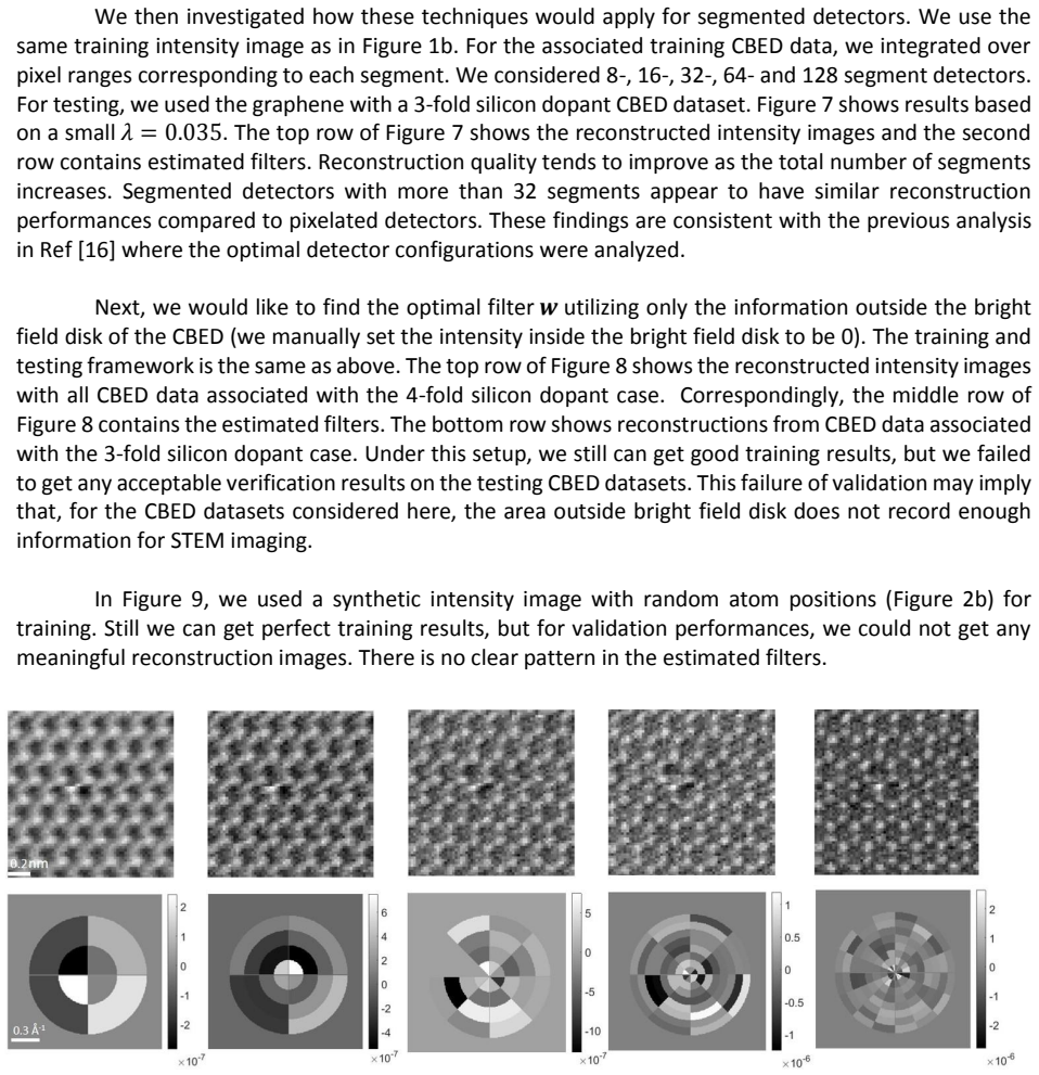
This paper establishes that direct inversion of the linear mapping $\boldsymbol{y} = X \boldsymbol{w}$ from vectorized convergent-beam electron diffraction (CBED) patterns to real-space image intensities is not merely noisy but systematically underdetermined: combinations of detector pixels exist that reproduce a prescribed training image with near-perfect fidelity while producing meaningless, non-transferable predictions elsewhere. The authors show this by training filters on artificial targets—excessively high resolution, random atom sites, ring patterns, and the word 'caveat'—and demonstrating that all fit the training half of the field of view yet fail on the other half. With elastic-net regularization over a path of sparsity strengths, they obtain filters that trade training fidelity for generalizable structure: at suitable values of the regularization parameter, reconstructed graphene dumbbells and dopant contrast match simultaneously acquired HAADF images, and the filters transfer to a second dataset with a different silicon dopant. They further find that bright-field disk information is sufficient, that outside-disk information fails validation, and that segmented detectors with 32 or more segments behave like full pixelated detectors.
Load-bearing premise
The paper assumes that a single fixed linear map from diffraction intensities to real-space image holds across all probe positions and across specimens, although real electron scattering is nonlinear and the training targets are themselves derived from the HAADF image used for validation.
Editorial extensions
If this is right
- Without held-out validation, one can deliberately construct filters that make a 4D-STEM dataset display arbitrarily high resolution, random atom sites, rings, or text-like patterns, so reported resolution claims are not self-certifying.
- Filter estimation on half a scan and prediction on the other half is a workable model-selection protocol; a filter that passes it reconstructs graphene structure comparably to HAADF imaging.
- For the graphene datasets studied, only the bright-field disk information survives validation; the region outside the disk, though rich in raw intensity, does not yield generalizable structure.
- Segmented detectors with about 32 segments or more reconstruct essentially as well as a full pixelated detector, connecting the statistical filter view to detector-design practice.
- Periodic training targets (complement of the atom image and individual sublattices) generalize under regularization, suggesting that crystal symmetry is a usable inductive bias for virtual imaging.
Reading between the lines
- The same overfitting hazard likely applies to black-box machine-learning models that map diffraction patterns to images; the paper's demonstration that a linear filter can reproduce the word 'caveat' is a minimal proof that any unregularized learned mapping can fit arbitrary targets.
- For amorphous or aperiodic samples, the paper's periodicity constraint would likely fail; a testable extension is to check whether symmetry-aware regularization, such as group sparsity on lattice sites, restores transferability.
- One could operationalize the paper's validation idea as a quantitative 'generalization index'—the ratio of test-area to training-area reconstruction error along the $\lambda$ path—and use it to select regularization automatically.
- Because a pixelated detector with a linear filter is mathematically a continuously segmented detector, the elastic-net filter landscape can be used to propose optimal discrete detector geometries for new STEM imaging modes.
Signed reviews
Editorial analysis
A structured set of objections, weighed in public.
Referee Report
Summary. The paper studies the risk of overfitting in 4D-STEM structure retrieval by treating real-space image formation as a linear regression on CBED intensities. It demonstrates that with n = 1,088 training samples and p = 65,536 CBED pixels, filters can be constructed via least squares to reproduce almost arbitrary training targets while failing on held-out data. The authors then apply elastic net regularization (Eq. 3) and claim that, with careful model selection and validation, robust filters can be obtained that yield images comparable to HAADF imaging. They also examine segmented detectors and the use of only the bright-field disk. The paper's main contribution is the cautionary demonstration of the flexibility and overfitting risk in high-dimensional diffraction data.
Significance. The negative result is convincing and practically important: the demonstration in Fig. 2 that arbitrary patterns (high-resolution lattices, random atom sites, rings, and the word 'caveat') can be fitted in-sample while failing in held-out regions is a clear warning to the 4D-STEM community. The numerical setup (n = 1,088, p = 65,536) makes the point starkly, and the comparison between pixelated and segmented detectors in Fig. 7 is interesting. However, the positive claim that regularization plus validation yields robust, HAADF-comparable filters is not quantitatively established. If the negative result is the main message, the paper is a useful cautionary note; if the positive claim is meant to be load-bearing, it needs substantially stronger validation.
major comments (4)
- [Formalism, Eqs. (1)-(2)] The paper assumes a fixed linear relationship y = Xw between vectorized CBED intensities and the real-space image, with no discussion of its validity under the experimental conditions. Dynamical diffraction, detector nonlinearity, sample drift, and the fact that the scattering depends on probe position may all violate this assumption. Since the positive claim of robust filter recovery depends on this linear model being at least approximately correct, the assumption needs justification or an explicit statement of its limitations.
- [Demonstrative Results, Eq. (3)] The paper claims to perform 'statistical model selection', but no model selection criterion is actually applied. The mixing parameter r is fixed at 5e-5 without sensitivity analysis, and λ is chosen by visual inspection of the reconstructions in Figs. 4-6 rather than by a quantitative criterion on validation data. The abstract's statement that 'careful choice of model selection and validation' yields robust filters is therefore not demonstrated by the presented analysis.
- [Demonstrative Results, Fig. 1b and Figs. 4-6] The training target image (Fig. 1b) is constructed from atom site positions estimated from the HAADF image in Fig. 1a, and the validation benchmark is the same HAADF image (or a HAADF image acquired under the same conditions). The comparison is therefore partly circular: the filter is trained on HAADF-derived lattice information and then evaluated for similarity to HAADF. An independent benchmark, such as known atomic coordinates from a simulation or a separately determined structure, is needed to support the claim of structure retrieval.
- [Demonstrative Results, Fig. 6b] The claimed 'comparable contrast to HAADF' is based on visual inspection and normalized line scans without quantitative similarity metrics or error bars. No mean-squared error, correlation coefficient, or Fourier ring correlation is reported on held-out data. Quantitative metrics are needed to support the claim that the reconstructed images are comparable to conventional HAADF imaging.
minor comments (5)
- [Abstract] The abstract contains grammatical issues, such as 'we demonstrate that, it is possible', and the affiliation includes a typo ('Laborotary').
- [Formalism] Equation (1) is referenced but missing from the text; the blank after 'the following linear relationship:' should contain the explicit form of the linear model.
- [Formalism] The phrase 'ordinary least square estimates' should be clarified, because with n < p the OLS solution is non-unique; the authors presumably mean the minimum-norm least-squares solution.
- [Demonstrative Results] The statement that varying r 'does not alter conclusions presented here' is not supported by any shown results; a small sensitivity analysis would make this claim credible.
- [Discussion] The reference to Ref. [33] for 'unsupervised learning and exploratory data analysis' should be checked for accuracy, since the cited paper is a manifold-learning study of 4D-STEM and the connection could be stated more precisely.
Circularity Check
No significant circularity: the overfitting demonstration and cross-sample filter transfer test are self-contained.
full rationale
The paper's derivation chain is not circular. It fits a linear filter w from CBED pixel intensities X to a user-specified real-space target y (Eqs. 1-3), then evaluates the fitted filter on held-out CBED data from the same sample (Fig. 4) and on a separately acquired dataset with a different dopant configuration (Fig. 5). The negative result, that arbitrary targets such as random atom sites, rings, or the word 'caveat' can be reproduced in the training region but fail on held-out data, is self-contained and directly demonstrates the overfitting pitfall. The positive result is a transfer test: a filter trained on atom-site targets derived from one HAADF image is applied to CBED from a different sample and compared to that sample's HAADF line profile; this is an external benchmark, not a restatement of the training target. The only self-citation (Ref. 33, 'unsupervised learning and exploratory data analysis') appears in a sentence about future work and is not load-bearing. The choice of lambda is made by visual inspection and no quantitative held-out metric is reported, which is a validation weakness, not circularity. Therefore no step satisfies the standard of being equivalent to its inputs by definition or by fitted-parameter renaming.
Assumptions & free parameters
free parameters (2)
- r (elastic net mixing parameter) =
5e-5
- lambda (regularization strength) =
decreasing sequence, values not all listed in text
assumptions (3)
- domain assumption A fixed linear filter w exists such that y = Xw (Eqs. 1-2) across all probe positions and samples.
- domain assumption CBED datasets collected under equivalent conditions share the same filter, allowing transfer from training to test samples.
- domain assumption The elastic net penalty is an appropriate prior for the filter w (sparsity/smoothness tradeoff).
Cite this review
Pith. "Pith review of Structure retrieval from 4D-STEM: statistical analysis of potential pitfalls in high-dimensional data." pith.science (2026). https://pith.science/paper/OW5IYCSN
@misc{pith2026190800659,
  author       = {Pith},
  title        = {Pith review of: Structure retrieval from 4D-STEM: statistical analysis of potential pitfalls in high-dimensional data},
  year         = {2026},
  howpublished = {\url{https://pith.science/paper/OW5IYCSN}},
  note         = {Machine review of arXiv:1908.00659}
}
read the original abstract
Four-dimensional scanning transmission electron microscopy (4D-STEM) is one of the most rapidly growing modes of electron microscopy imaging. The advent of fast pixelated cameras and the associated data infrastructure have greatly accelerated this process. Yet conversion of the 4D datasets into physically meaningful structure images in real-space remains an open issue. In this work, we demonstrate that, it is possible to systematically create filters that will affect the apparent resolution or even qualitative features of the real-space structure image, reconstructing artificially generated patterns. As initial efforts, we explore statistical model selection algorithms, aiming for robustness and reliability of estimated filters. This statistical model selection analysis demonstrates the need for regularization and cross-validation of inversion methods to robustly recover structure from high-dimensional diffraction datasets.
Figures


Figures from the paper (6 more)




Reference graph
Works this paper leans on
-
[1]
T. J. Pennycook, A. R. Lupini, H. Yang, M. F. Murfitt, L. Jones, and P. D. Nellist, “Efficient phase contrast imaging in STEM using a pixelated detector. Part 1: Experimental demonstration at atomic resolution,” Ultramicroscopy, vol. 151, pp. 160–167, Apr. 2015
work page 2015
-
[2]
C. Ophus et al., “Efficient linear phase contrast in scanning transmission electron microscopy with matched illumination and detector interferometry,” Nat. Commun., vol. 7, p. 10719, Feb. 2016
work page 2016
-
[3]
High Dynamic Range Pixel Array Detector for Scanning Transmission Electron Microscopy,
M. W. Tate et al., “High Dynamic Range Pixel Array Detector for Scanning Transmission Electron Microscopy,” Microsc. Microanal., vol. 22, no. 01, pp. 237–249, Feb. 2016
work page 2016
-
[4]
PHASE CONTRAST IN SCANNING TRANSMISSION ELECTRON MICROSCOPY.,
H. Rose, “PHASE CONTRAST IN SCANNING TRANSMISSION ELECTRON MICROSCOPY.,” Optik (Stuttg)., vol. 39, pp. 416–436, 1974
work page 1974
-
[5]
DIFFERENTIAL PHASE CONTRAST IN A STEM.,
N. H. Dekkers and H. de Lang, “DIFFERENTIAL PHASE CONTRAST IN A STEM.,” Optik (Stuttg)., vol. 41, no. 4, pp. 452–456, 1974
work page 1974
-
[6]
Visualization of Light Elements at Ultrahigh Resolution by STEM Annular Bright Field Microscopy,
E. Okunishi, I. Ishikawa, H. Sawada, F. Hosokawa, M. Hori, and Y. Kondo, “Visualization of Light Elements at Ultrahigh Resolution by STEM Annular Bright Field Microscopy,” Microsc. Microanal., vol. 15, no. S2, pp. 164–165, Jul. 2009
work page 2009
-
[7]
Dynamics of annular bright field imaging in scanning transmission electron microscopy.,
S. D. Findlay, N. Shibata, H. Sawada, E. Okunishi, Y. Kondo, and Y. Ikuhara, “Dynamics of annular bright field imaging in scanning transmission electron microscopy.,” Ultramicroscopy, vol. 110, no. 7, pp. 903–23, Jun. 2010
work page 2010
-
[8]
Direct imaging of hydrogen-atom columns in a crystal by annular bright-field electron microscopy,
R. Ishikawa, E. Okunishi, H. Sawada, Y. Kondo, F. Hosokawa, and E. Abe, “Direct imaging of hydrogen-atom columns in a crystal by annular bright-field electron microscopy,” Nat. Mater., vol. 10, no. 4, p. 278, 2011
work page 2011
Show all 33 references
-
[9]
Differential phase contrast microscopy of magnetic materials,
J. N. Chapman, R. Ploessl, and D. M. Donnet, “Differential phase contrast microscopy of magnetic materials,” Ultramicroscopy, vol. 47, no. 4, pp. 331–338, 1992
1992
-
[10]
Differential phase- contrast microscopy at atomic resolution,
N. Shibata, S. D. Findlay, Y. Kohno, H. Sawada, Y. Kondo, and Y. Ikuhara, “Differential phase- contrast microscopy at atomic resolution,” Nat. Phys., vol. 8, no. 8, pp. 611–615, Aug. 2012
2012
-
[11]
Differential phase contrast 2.0—Opening new ‘fields’ for an established technique,
M. Lohr et al., “Differential phase contrast 2.0—Opening new ‘fields’ for an established technique,” Ultramicroscopy, vol. 117, pp. 7–14, Jun. 2012
2012
-
[12]
Nonstandard imaging methods in electron microscopy.,
H. Rose, “Nonstandard imaging methods in electron microscopy.,” Ultramicroscopy, vol. 2, no. 2– 3, pp. 251–67, Apr. 1977
1977
-
[13]
Enhanced light element imaging in atomic resolution scanning transmission electron microscopy,
S. D. Findlay, Y. Kohno, L. A. Cardamone, Y. Ikuhara, and N. Shibata, “Enhanced light element imaging in atomic resolution scanning transmission electron microscopy,” Ultramicroscopy, vol. 136, pp. 31–41, 2014
2014
-
[14]
Direct Visualization of Local Electromagnetic Field Structures by Scanning Transmission Electron Microscopy,
N. Shibata et al., “Direct Visualization of Local Electromagnetic Field Structures by Scanning Transmission Electron Microscopy,” Acc. Chem. Res., vol. 50, no. 7, pp. 1502–1512, 2017
2017
-
[15]
Experimental tests on double-resolution coherent imaging via STEM,
J. M. Rodenburg, B. C. McCallum, and P. D. Nellist, “Experimental tests on double-resolution coherent imaging via STEM,” Ultramicroscopy, vol. 48, no. 3, pp. 304–314, 1993
1993
-
[16]
Efficient phase contrast imaging in STEM using a pixelated detector. Part II: Optimisation of imaging conditions,
H. Yang, T. J. Pennycook, and P. D. Nellist, “Efficient phase contrast imaging in STEM using a pixelated detector. Part II: Optimisation of imaging conditions,” Ultramicroscopy, vol. 151, pp. 232–239, 2015
2015
-
[17]
Structure retrieval with fast electrons using segmented detectors,
H. G. Brown et al., “Structure retrieval with fast electrons using segmented detectors,” Phys. Rev. B, vol. 93, no. 13, p. 134116, 2016
2016
-
[18]
Atomic electric fields revealed by a quantum mechanical approach to electron picodiffraction,
K. Müller et al., “Atomic electric fields revealed by a quantum mechanical approach to electron picodiffraction,” Nat. Commun., vol. 5, p. 5653, Dec. 2014
2014
-
[19]
Measurement of atomic electric fields and charge densities from average momentum transfers using scanning transmission electron microscopy,
K. Müller-Caspary et al., “Measurement of atomic electric fields and charge densities from average momentum transfers using scanning transmission electron microscopy,” Ultramicroscopy, vol. 178, pp. 62–80, 2017
2017
-
[20]
Towards quantitative, atomic-resolution reconstruction of the electrostatic potential via differential phase contrast using electrons,
R. Close, Z. Chen, N. Shibata, and S. D. Findlay, “Towards quantitative, atomic-resolution reconstruction of the electrostatic potential via differential phase contrast using electrons,” Ultramicroscopy, vol. 159, pp. 124–137, 2015
2015
-
[21]
Quantitative electric field mapping in thin specimens using a segmented detector: Revisiting the transfer function for differential phase contrast,
T. Seki, G. Sánchez-Santolino, R. Ishikawa, S. D. Findlay, Y. Ikuhara, and N. Shibata, “Quantitative electric field mapping in thin specimens using a segmented detector: Revisiting the transfer function for differential phase contrast,” Ultramicroscopy, vol. 182, pp. 258–263, 2017
2017
-
[22]
Theoretical Framework of Statistical Noise in Scanning Transmission Electron Microscopy,
T. Seki, Y. Ikuhara, and N. Shibata, “Theoretical Framework of Statistical Noise in Scanning Transmission Electron Microscopy,” Ultramicroscopy, 2018
2018
-
[23]
Mitigating e-beam-induced hydrocarbon deposition on graphene for atomic-scale scanning transmission electron microscopy studies,
O. Dyck, S. Kim, S. V. Kalinin, and S. Jesse, “Mitigating e-beam-induced hydrocarbon deposition on graphene for atomic-scale scanning transmission electron microscopy studies,” J. Vac. Sci. Technol. B, Nanotechnol. Microelectron. Mater. Process. Meas. Phenom., vol. 36, no. 1, ...
2018
-
[24]
Placing single atoms in graphene with a scanning transmission electron microscope,
O. Dyck, S. Kim, S. V. Kalinin, and S. Jesse, “Placing single atoms in graphene with a scanning transmission electron microscope,” Appl. Phys. Lett., vol. 111, no. 11, p. 113104, Sep. 2017
2017
-
[25]
Regularization and variable selection via the elastic net,
H. Zou and T. Hastie, “Regularization and variable selection via the elastic net,” J. R. Stat. Soc. Ser. B (Statistical Methodol., vol. 67, no. 2, pp. 301–320, 2005
2005
-
[26]
Regression shrinkage and selection via the lasso,
R. Tibshirani, “Regression shrinkage and selection via the lasso,” J. R. Stat. Soc. Ser. B, pp. 267– 288, 1996
1996
-
[27]
Pathwise coordinate optimization,
J. Friedman, T. Hastie, H. Höfling, R. Tibshirani, and others, “Pathwise coordinate optimization,” Ann. Appl. Stat., vol. 1, no. 2, pp. 302–332, 2007
2007
-
[28]
Regularization paths for generalized linear models via coordinate descent,
J. Friedman, T. Hastie, and R. Tibshirani, “Regularization paths for generalized linear models via coordinate descent,” J. Stat. Softw., vol. 33, no. 1, p. 1, 2010
2010
-
[29]
Direct Determination of the Chemical Bonding of Individual Impurities in Graphene,
W. Zhou, M. D. Kapetanakis, M. P. Prange, S. T. Pantelides, S. J. Pennycook, and J.-C. Idrobo, “Direct Determination of the Chemical Bonding of Individual Impurities in Graphene,” Phys. Rev. Lett., vol. 109, no. 20, p. 206803, Nov. 2012
2012
-
[30]
Probing the Bonding and Electronic Structure of Single Atom Dopants in Graphene with Electron Energy Loss Spectroscopy,
Q. M. Ramasse, C. R. Seabourne, D.-M. Kepaptsoglou, R. Zan, U. Bangert, and A. J. Scott, “Probing the Bonding and Electronic Structure of Single Atom Dopants in Graphene with Electron Energy Loss Spectroscopy,” Nano Lett., vol. 13, no. 10, pp. 4989–4995, Oct. 2013
2013
-
[31]
Sparse regression with exact clustering,
Y. She, “Sparse regression with exact clustering,” Electron. J. Stat., vol. 4, pp. 1055–1096, 2010
2010
-
[32]
Structured Variable Selection with Sparsity-Inducing Norms,
R. Jenatton, J.-Y. Audibert, and F. Bach, “Structured Variable Selection with Sparsity-Inducing Norms,” J. Mach. Learn. Res., vol. 12, no. Oct, pp. 2777–2824, 2011
2011
-
[33]
Manifold learning of four-dimensional scanning transmission electron microscopy,
X. Li et al., “Manifold learning of four-dimensional scanning transmission electron microscopy,” npj Comput. Mater., vol. 5, no. 1, p. 5, 2019
2019
Reviewed August 14, 2026 · model on record in the stance chip above.
Discussion (0). Continue with ORCID to comment.