REVIEW 3 major objections 5 minor 50 references
Population Predictive Checks
T0 review · 3 major / 5 minor · reviewed 2026-08-14 · deepseek-v4-flash
Pith's one-line read The population predictive check evaluates a Bayesian model on fresh draws from the population, and the paper proves this check is properly calibrated.
desk verdict The paper's headline claim—that Pop-PCs are properly calibrated—is false even in a correct normal model; the framework is still interesting but needs major rework. read the letter →
The pith
A machine-rendered reading of the paper's core claim, the machinery that carries it, and where it could break.
The reading
What carries the argument
The central object is the ideal population predictive check, $\mathrm{Pop\text{-}PC}(y_{\text{obs}}, F; d, g) = \mathbb{E}[g(d(Y_{\text{rep}}), d(Y_{\text{new}})) \mid y_{\text{obs}}, F]$, where $Y_{\text{rep}}$ is drawn from the posterior predictive and $Y_{\text{new}}$ from the population. The machinery is the separation it enforces between the conditioning data and the evaluation data: with $g(a,b) = \mathbb{1}[a > b]$, this becomes a tail probability whose reference distribution is $F$ rather than the observed data, which is what makes the p-value uniform under a correct model. Finite-data implementations replace $F$ with the empirical distribution and obtain $(y_{\text{obs}}, y_{\text{new}})$ by cross-validation, bootstrap, out-of-bag, or double-bootstrap sampling, refitting the posterior on each resampled $y_{\text{obs}}$.
What would settle it
Simulate many datasets from a known Bayesian model, run Algorithm 1 on each with the bootstrap estimator, and check whether the resulting Pop-PC p-values are approximately uniform; a systematic deviation would show the practical check is not properly calibrated.
Extended reading notes
Core claim
The central discovery is that the reference distribution in a Bayesian model check should be the population distribution, not the observed data. The population predictive p-value, $p(d(Y_{\text{rep}}) > d(Y_{\text{new}}) \mid y_{\text{obs}}, F)$, compares a discrepancy computed on posterior-predictive replicates with the same discrepancy computed on fresh data from the population. Because $Y_{\text{new}}$ is drawn independently of the conditioning data, this p-value has a uniform reference distribution under a correct model; the posterior predictive p-value, which compares replicates with the observed data, does not. The paper extends this idea to realized discrepancies that depend on latent variables and to per-group checks in hierarchical models.
Load-bearing premise
The practical routines assume that resampling the data you already have can stand in for drawing genuinely new data from the real population, and the paper does not prove that this estimated check keeps the ideal check's calibration.
Editorial extensions
If this is right
- If the model is correct, Pop-PC p-values are uniform, so the check will not systematically over-reject or under-reject; posterior predictive p-values cluster around one-half and lack this calibration.
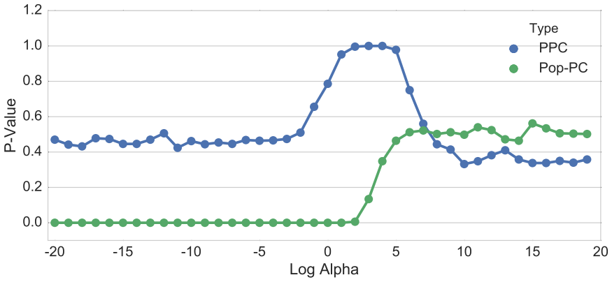
- Pop-PCs will not reward a model that memorizes its training data, because fresh population draws will not match the memorized distribution; the Dirichlet-process example shows a PPC preferring the empirical distribution while the Pop-PC gives extreme p-values for the same misfit.
- The bootstrap and cross-validation estimators are practical with any posterior approximation and, in the regression experiments, follow the ideal Pop-PC as model flexibility grows, whereas the PPC prefers more flexible models.
- In the hierarchical topic model, the Pop-PC detects the memorization pathology as the number of topics grows, with orders of magnitude more deviance than the PPC.
- The construction covers realized discrepancies and hierarchical models, so checks can target individual groups or latent-variable structure rather than only whole datasets.
Reading between the lines
- The calibration guarantee is stated for the ideal check that samples from the true population; the empirical estimators swap in the empirical distribution, so whether each estimator inherits uniformity under the null is an open question that the paper does not resolve.
- The same 'evaluate on fresh population draws' move could be applied to other diagnostics that currently use the observed data as their reference, such as surprise measures for outlier detection, giving them uniform calibration as well.
- Because Algorithm 1 refits the posterior for every resampled dataset, practical scaling will require amortized inference or approximate refits; the paper mentions bag-of-little-bootstraps but does not analyze the statistical cost of reusing a single posterior fit.
Signed reviews
Editorial analysis
A structured set of objections, weighed in public.
Referee Report
Summary. The paper introduces the population predictive check (Pop-PC), a model criticism procedure that replaces the reference data in a posterior predictive check (PPC) by a draw from the true population distribution. Section 3 defines an ideal Pop-PC (Eqs. 7 and 9), in which replicated data from the posterior predictive distribution are compared with new data from the population distribution F, and Section 4 proposes bootstrap, cross-validation, double-bootstrap, and p-bootstrap estimators that approximate F with the empirical distribution of the observed sample. Section 3.4 extends the construction to realized discrepancies and to hierarchical models with local latent variables. The abstract claims that, unlike the PPC, the Pop-PC is 'properly calibrated'; the paper presents empirical studies on Bayesian linear regression and a topic model suggesting that Pop-PCs detect overfitting where PPCs do not.
Significance. The idea of checking a posterior predictive distribution against a reference or held-out population is natural, and the paper's taxonomy of bootstrap and cross-validation estimators is clearly presented and potentially useful. If the calibration claim were true, the paper would address a well-known limitation of posterior predictive checks and supply interpretable p-values. The empirical demonstrations are suggestive. However, the central theoretical claim is not proved anywhere in the manuscript, and under the paper's own definition of interpretable p-values it is false: the ideal Pop-PC p-value of Eq. 9 is not uniform even in a correctly specified location model. Because this claim is the advertised contribution and is the basis for the practical estimators in Section 4, the manuscript does not establish its central thesis.
major comments (3)
- [Abstract; Section 3.1, p. 8; Section 3.2, Eq. (9)] The abstract states that 'we prove that the Pop-PC is properly calibrated,' and Section 3.1 defines interpretable p-values as those with a uniform reference distribution, citing Robins et al. (2000). No theorem or proof of uniformity appears in Section 3.2 or anywhere else, and the statement is false under the paper's own definition. Consider the correctly specified model y|μ∼N(μ,1), μ∼N(0,1), population F=N(0,1), n=1, and discrepancy d(y)=y. The posterior predictive is Yrep|yobs∼N(yobs/2, 3/2), and Ynew∼N(0,1). Eq. (9) gives p_ideal(yobs,F)=P(Yrep>Ynew|yobs,F)=Φ(0.316·yobs). Over yobs∼F, this equals Φ(0.316Z) with Z∼N(0,1), so P(p≤0.05)≈10^{-7}, not 0.05. If instead one conditions on the sampled held-out ynew, as Algorithm 1 does, the p-value is Φ(0.913Z), which is also not uniform. Thus the ideal Pop-PC is not properly calibrated under the standard stated in Section 3.1, and the bootstrap/CV estimators in Section 4 cannot inherit a property the ideal check does not have.
- [Section 4, Algorithm 1 and surrounding text] The estimators replace the population F with the empirical distribution of the finite pool y and resample both yobs and ynew from y, but no analysis is provided for the resulting p-value's reference distribution. In Algorithm 1, θ is drawn from p(θ|yobs) where yobs is a bootstrap or cross-validation subsample of y, so the posterior and the reference data are dependent through the same finite pool; this is a different object from the ideal check of Eq. (7). The paper asserts that the bootstrap and cross-validation variants approximate the ideal check and that the 632 estimator is closest in simulation, but it supplies no consistency, asymptotic-uniformity, or calibration result for any variant. Consequently, the practical claim that the computed checks are 'properly calibrated' is not established, and the simulation evidence in Section 5 cannot substitute for this missing theory.
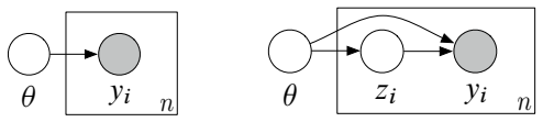
- [Section 3.4, Eq. (14); Section 5.2] The per-group realized-discrepancy check draws znew_j from p(z|yobs_j, θ) while ynew_j is drawn from F_j, so znew_j and ynew_j are not generated from a common model; the distribution of d(Ynew_j, Znew_j, θ) is neither a posterior predictive draw nor a pure population draw. No property of this mixed distribution is stated, and it is unclear what calibration statement, if any, is intended. This matters because the LDA experiment in Section 5.2 uses exactly this local-variable construction with the IMI discrepancy, so the empirical comparison between PPC and Pop-PC rests on an object whose statistical behavior is not analyzed.
minor comments (5)
- [Abstract] The phrase 'frequenting assessment' appears to be a typo for 'frequentist assessment.'
- [Section 3.3, Eq. (11)] The discrepancy d(y)= (1/n) Σ log p(y_i | yobs) depends on the observed data through p(y_i|yobs), which is itself a function of the full observed set; this unusual definition should be clarified because it introduces a second, less obvious use of yobs inside the discrepancy.
- [Figures 2, 4, and 5] The plots show point values of p-values or discrepancies without error bars, repeated-simulation variability, or uncertainty quantification; claims such as 'the 632 Bootstrap estimator is closest to the ideal check' are not supported quantitatively.
- [References] The entries Tran et al. (2016a) and Tran et al. (2016b) are identical and should be merged or distinguished.
- [Section 5.2] The IMI discrepancy is attributed to Mimno and Blei (2011) but the formula in the text is incomplete (it leaves the indexing of words and documents implicit), and no derivation or computation details are given; an appendix with the exact estimator would improve reproducibility.
Circularity Check
No circular derivation; the calibration claim is asserted, not derived, but no step reduces to its own input.
full rationale
The paper's central definition, the ideal Pop-PC in Eqs. 7-9, is an expectation comparing replicated data drawn from the posterior predictive to new data drawn from the population distribution. No parameter is fit to the target claim, no output quantity is renamed from an input, and no equation is equal to another by construction. The abstract's statement that 'we prove that the Pop-PC is properly calibrated' is not supported by a proof in Sections 3.2-4, and the uniformity of the Eq. 9 p-value is not established; this is a missing proof and a correctness risk, not a circularity. The bootstrap and cross-validation estimators in Section 4 are asserted to approximate the ideal check without an analysis of estimation error, which is an unproven approximation assumption rather than a circular reduction. The self-citations to Mimno and Blei (2011) for the topic-model discrepancy and to Blei et al. (2003) for LDA are illustrative experimental inputs, not load-bearing premises of the method's derivation. Overall, no significant circularity is present.
Assumptions & free parameters
assumptions (4)
- domain assumption Data are i.i.d. draws from an unknown population distribution F.
- domain assumption The empirical distribution (plug-in principle) approximates the population distribution well enough for bootstrap and cross-validation estimators.
- domain assumption The posterior distribution p(theta | yobs) is available through MCMC or variational inference.
- domain assumption For hierarchical models, local latent variables z drawn from p(z | y_j, theta) explain new data from the same group.
Cite this review
Pith. "Pith review of Population Predictive Checks." pith.science (2026). https://pith.science/paper/QOA2XXR5
@misc{pith2026190800882,
  author       = {Pith},
  title        = {Pith review of: Population Predictive Checks},
  year         = {2026},
  howpublished = {\url{https://pith.science/paper/QOA2XXR5}},
  note         = {Machine review of arXiv:1908.00882}
}
read the original abstract
Bayesian modeling helps applied researchers articulate assumptions about their data and develop models tailored for specific applications. Thanks to good methods for approximate posterior inference, researchers can now easily build, use, and revise complicated Bayesian models for large and rich data. These capabilities, however, bring into focus the problem of model criticism. Researchers need tools to diagnose the fitness of their models, to understand where they fall short, and to guide their revision. In this paper we develop a new method for Bayesian model criticism, the population predictive check (Pop-PC). Pop-PCs are built on posterior predictive checks (PPCs), a seminal method that checks a model by assessing the posterior predictive distribution on the observed data. However, PPCs use the data twice -- both to calculate the posterior predictive and to evaluate it -- which can lead to overconfident assessments of the quality of a model. Pop-PCs, in contrast, compare the posterior predictive distribution to a draw from the population distribution, a heldout dataset. This method blends Bayesian modeling with frequenting assessment. Unlike the PPC, we prove that the Pop-PC is properly calibrated. Empirically, we study Pop-PC on classical regression and a hierarchical model of text data.
Figures

Figures from the paper (3 more)


Reference graph
Works this paper leans on
-
[1]
Handbook of Mixed Membership Models and Their Applications
Airoldi, E., Blei, D., Erosheva, E., and Fienberg, S., editors (2014). Handbook of Mixed Membership Models and Their Applications . CRC Press
work page 2014
-
[2]
Angelino, E., Johnson, M., and Adams, R. (2016). Patterns of scalable B ayesian inference. Foundations and Trends in Machine Learning , 9(2-3):119--247
work page 2016
-
[3]
Bayarri, M. and Berger, J. (2000). P-values for composite null models. Journal of the American Statistical Association , 95(452):1127--1142
work page 2000
-
[4]
Bayarri, M. and Castellanos, M. (2007). Bayesian checking of the second levels of hierarchical models. Statistical Science , 22:322--343
work page 2007
-
[5]
Bayarri, M. and Morales, J. (2003). Bayesian measures of surprise for outlier detection. Journal of Statistical Planning and Inference , 111:3--22
work page 2003
-
[6]
Beaumont, M., Zhang, W., and Balding, D. (2002). Approximate B ayesian computation in population genetics. Genetics , 162(4):2025--2035
work page 2002
-
[7]
Belin, T. and Rubin, D. (1995). The analysis of repeated-measures data on schizophrenic reaction times using mixture models. Statistics in Medicine , 14(8):747--768
work page 1995
-
[8]
Blei, D. (2014). Build, compute, critique, repeat: D ata analysis with latent variable models. Annual Review of Statistics and Its Application , 1:203--232
work page 2014
Show all 50 references
-
[9]
Blei, D., Kucukelbir, A., and McAuliffe, J. (2017). Variational inference: A review for statisticians. Journal of American Statistical Association , 112(518):859--877
2017
-
[10]
Blei, D., Ng, A., and Jordan, M. (2003). Latent D irichlet allocation. Journal of Machine Learning Research , 3:993--1022
2003
-
[11]
Box, G. (1980). Sampling and B ayes' inference in scientific modeling and robustness. Journal of the Royal Statistical Society, Series A , 143(4):383--430
1980
-
[12]
Breiman, L. (1996). Out-of-bag estimation. Technical report, Statistics Department, U.C. Berkeley
1996
-
[13]
D., Lee, D., Goodrich, B., Betancourt, M., Brubaker, M., Guo, J., Li, P., and Riddell, A
Carpenter, B., Gelman, A., Hoffman, M. D., Lee, D., Goodrich, B., Betancourt, M., Brubaker, M., Guo, J., Li, P., and Riddell, A. (2016). Stan: A probabilistic programming language. Journal of Statistical Software
2016
-
[14]
Chatfield, C. (1995). Model uncertainty, data mining and statistical inference. Journal of the Royal Statistical Society. Series A (Statistics in Society) , 158(3):419--466
1995
-
[15]
Dahl, F., G semyr, J., and Natvig, B. (2007). A robust conflict measure of inconsistencies in bayesian hierarchical models. Scandinavian Journal of Statistics , 34(4):816--828
2007
-
[16]
Dey, D., Gelfand, A., Swartz, T., and Vlachos, P. (1998). Simulation based model checking for hierarchical models. Test
1998
-
[17]
Draper, D. (1996). Comment: U tility,sensitivity analysis, and cross-validation in bayesian model-checking. Statistica Sinica , 6(760--767.)
1996
-
[18]
Efron, B. (1979). Bootstrap methods: A nother look at the jackknife. The Annals of Statistics , pages 1--26
1979
-
[19]
and Tibshirani, R
Efron, B. and Tibshirani, R. (1993). An Introduction to the Bootstrap . Chapman & Hall
1993
-
[20]
and Tibshirani, R
Efron, B. and Tibshirani, R. (1997). Improvements on cross-validation: T he 632+ bootstrap method. Journal of the American Statistical Association , 92(438):548--560
1997
-
[21]
Ferguson, T. (1973). A B ayesian analysis of some nonparametric problems. The Annals of Statistics , 1:209--230
1973
-
[22]
Geisser, S. (1975). The predictive sample reuse method with applications. Journal of the American Statistical Association , 70(350):320--328
1975
-
[23]
Gelfand, A., Dey, D., and Chang, H. (1992). Model determination using predictive distributions with implementation via sampling-based methods. Bayesian Statistics , 4
1992
-
[24]
Gelman, A., Carlin, J., Stern, H., and Rubin, D. (1995). Bayesian Data Analysis . Chapman & Hall, London
1995
-
[25]
and Hill, J
Gelman, A. and Hill, J. (2007). Data Analysis Using Regression and Multilevel/Hierarchical Models . Cambridge University Press
2007
-
[26]
Gelman, A., Meng, X., and Stern, H. (1996). Posterior predictive assessment of model fitness via realized discrepancies. Statistica Sinica , 6:733--807
1996
-
[27]
and Stuhlmuller, A
Goodman, N. and Stuhlmuller, A. (2015). The design and implementation of probabilistic programming languages
2015
-
[28]
Guttman, I. (1967). The use of the concept of a future observation in goodness-of-fit problems. Journal of the Royal Statistical Society. Series B (Methodological) , pages 83--100
1967
-
[29]
Hjort, N., Dahl, F., and Steinbakk, G. (2006). Post-processing posterior predictive p values. Journal of the American Statistical Association , 101(475):1157--1174
2006
-
[30]
Hjort, N., Holmes, C., Mueller, P., and Walker, S. (2010). Bayesian Nonparametrics: Principles and Practice . Cambridge University Press, Cambridge, UK
2010
-
[31]
Hoffman, M., Blei, D., Wang, C., and Paisley, J. (2013). Stochastic variational inference. Journal of Machine Learning Research , 14(1303--1347)
2013
-
[32]
and Gelman, A
Hoffman, M. and Gelman, A. (2014). The no- U -turn sampler: A daptively setting path lengths in H amiltonian M onte C arlo. Journal of Machine Learning Research , 15(1):1593--1623
2014
-
[33]
Kleiner, A., Talwalkar, A., Sarkar, P., and Jordan, M. (2012). A scalable bootstrap for massive data. arXiv":1112.5016
2012 arXiv
-
[34]
and Raftery, A
Lewis, S. and Raftery, A. (1996). Comment: P osterior predictive assessment for data subsets in hierarchical models via MCMC . Statistica Sinica , 6:779--786
1996
-
[35]
Mansinghka, V., Selsam, D., and Perov, Y. (2014). Venture: A higher-order probabilistic programming platform with programmable inference. arXiv:1404.0099
2014 arXiv
-
[36]
and Spiegelhalter, D
Marshall, E. and Spiegelhalter, D. (2003). Approximate cross-validatory predictive checks in disease mapping models. Statistics in Medicine , 22:1649--1660
2003
-
[37]
Meng, X.-L. (1994). Posterior predictive p-values. The Annals of Statistics , pages 1142--1160
1994
-
[38]
and Blei, D
Mimno, D. and Blei, D. (2011). Bayesian checking for topic models. In Empirical Methods in Natural Language Processing
2011
-
[39]
Mimno, D., Blei, D., and Engelhardt, B. (2015). Posterior predictive checks to quantify lack-of-fit in admixture models of latent population structure. Proceedings of the National Academy of Sciences
2015
-
[40]
O'Hagan, A. (2003). H SSS model criticism. In Highly Structured Stochastic Systems , volume 27 of Oxford Statist. Sci. Ser. , pages 423--453. Oxford Univ. Press, Oxford
2003
-
[41]
Ranganath, R., Gerrish, S., and Blei, D. (2014). Black box variational inference. In Artificial Intelligence and Statistics , pages 814--822
2014
-
[42]
Robins, J., van der Vaart, A., and Ventura, V. (2000). Asymptotic distribution of p -values in composite null models. Journal of the American Statistical Association , 95(452):1143--1156
2000
-
[43]
Rubin, D. (1984). Bayesianly justifiable and relevant frequency calculations for the applied statistician. The Annals of Statistics , 12(4):1151--1172
1984
-
[44]
and Mnih, A
Salakhutdinov, R. and Mnih, A. (2008). Probabilistic matrix factorization. In Neural Information Processing Systems
2008
-
[45]
Srivastava, S., Li, C., and Dunson, D. (2018). Scalable B ayes via barycenter in W asserstein space. The Journal of Machine Learning Research , 19(1):312--346
2018
-
[46]
Stan: A C ++ library for probability and sampling, version 2.8.0
Stan Development Team (2015). Stan: A C ++ library for probability and sampling, version 2.8.0
2015
-
[47]
Stone, M. (1974). Cross-validatory choice and assessment of statistical predictions. Journal of the Royal Statistical Society. Series B (Methodological) , pages 111--147
1974
-
[49]
B., Rudolph, M., Liang, D., and Blei, D
Tran, D., Kucukelbir, A., Dieng, A. B., Rudolph, M., Liang, D., and Blei, D. M. (2016b). Edward: A library for probabilistic modeling, inference, and criticism. arXiv:1610.09787
2016 arXiv
-
[50]
Vehtari, A., Gelman, A., and Gabry, J. (2016). Practical B ayesian model evaluation using leave-one-out cross-validation and WAIC . Statistics and Computing
2016
-
[51]
Wood, F., van de Meent, J.-W., and Mansinghka, V. (2014). A new approach to probabilistic programming inference. In Artificial Intelligence and Statistics , pages 1024--1032
2014
Reviewed August 14, 2026 · model on record in the stance chip above.
Discussion (0). Continue with ORCID to comment.