Linear Dynamics: Clustering without identification

Chloe Ching-Yun Hsu; Michaela Hardt; Moritz Hardt

REVIEW 4 major objections 4 minor 12 references

Linear Dynamics: Clustering without identification

T0 review · 4 major / 4 minor · reviewed 2026-08-14 · deepseek-v4-flash

Challenge this review Re-run · record.json Download PDF Read on arXiv ↗ Review JSON

Pith's one-line read Outputs alone reveal eigenvalues of hidden linear dynamics

desk verdict Useful practical method for LDS eigenvalue estimation and clustering; the headline convergence rate is over-stated, and Theorem 4.2 has a reciprocal-polynomial bug that is easy to fix but should not be left as is. read the letter →

arxiv 1908.01039 v3 pith:CPI3O4DG submitted 2019-08-02 cs.LG stat.ML

Chloe Ching-Yun Hsu , Michaela Hardt , Moritz Hardt This is my paper · ORCID

classification cs.LGstat.ML MSC 93B3062M1015A18

keywords lineardynamicalsystemseigenspectrumidentificationARMAmodelsautoregressiveparametersiteratedregressiontimeseriesclusteringobservabilitysystem

verification ladder T0 review T1 audit T2 compute T3 formal

The pith

A machine-rendered reading of the paper's core claim, the machinery that carries it, and where it could break.

The reading

This paper establishes that the eigenvalues of the state-transition matrix in a linear dynamical system can be identified from the observed output series alone, even when the full system parameters cannot be recovered. The mechanism is an exact correspondence: each dimension of the output obeys an ARMAX model whose autoregressive coefficients are, up to sign, the coefficients of the characteristic polynomial of the transition matrix. A regularized iterated least-squares regression estimates those coefficients consistently, converging at rate O($T^{{-1/2}}$) in the sequence length. Because eigenvalues characterize the dynamics up to change of basis, the fitted autoregressive parameters become a natural, computationally cheap similarity measure for clustering time series, including series of different lengths, with temporal offsets, or recorded by different measurement procedures. The paper demonstrates the approach on simulated linear dynamical system data and on electrocardiogram recordings, where it matches or improves clustering quality relative to existing baselines.

What carries the argument

The reciprocal characteristic polynomial χ†_A(L) = L^n χ_A($L^{{-1}}$), applied as a lag-operator polynomial, is the load-bearing identity. The proof expands the hidden state in a Jordan canonical basis of the adjoint A^*, showing that applying (1−λL)^μ to a projected state leaves only a linear combination of past inputs; multiplying over all eigenvalues gives χ†_A(L) y_t as a linear combination of past inputs plus noise. This is what makes the characteristic polynomial of A literally equal to the autoregressive polynomial of the output series. On the estimation side, the companion matrix of the estimated AR polynomial carries the argument: parameter error becomes matrix perturbation, and eigenvalue perturbation bounds (regular splitting for repeated roots, Vandermonde-based explicit bounds for simple roots) convert AR estimation error into eigenvalue error.

What would settle it

Run the estimator on output from a deliberately unobservable system, such as one where a tightly damped eigenmode is orthogonal to the measurement matrix C; the recovered spectrum should miss that mode, matching the paper's own observability caveat. Alternatively, generate a system with a double eigenvalue and perturb the fitted AR coefficients by ε; the two estimated roots should separate at rate √ε rather than ε, as the general O($ε^{{1/2}}$) bound predicts.

Watch

Extended reading notes

Core claim

The central discovery is that the eigenspectrum of the unknown transition matrix A is readable from the output series without identifying B, C, or D. Theorem 4.1 shows that, for an n-dimensional linear dynamical system, every output dimension is generated by an ARMAX(n, n, n−1) model whose autoregressive parameters φ1, ..., φn satisfy χ_A(λ) = λ^n − φ1 $λ^{{n−1}}$ − ⋯ − φn; in the no-input case the model reduces to an ARMA(n, n) process. Consequently, two output series share the same autoregressive parameters if and only if the underlying systems have the same nonzero eigenvalues with the same multiplicities (Corollary 4.1). The paper pairs this with perturbation results: an ε error in the autoregressive parameters leads to O($ε^{{1/n}}$) eigenvalue error in general, and O(ε) when all eigenvalues are simple, with an explicit condition-number bound for the latter case. Joined with a consistent iterated-regression estimator of ARMA autoregressive parameters, this yields an O($T^{{−1/2}}$) estimator of the eigenvalues of A from outputs alone.

Load-bearing premise

The load-bearing premise is that the system is observable — every hidden mode leaves a trace in the output — and that no pole-zero cancellation, no hidden cancellation between the AR and MA parts, reduces the effective order; if either fails, the output follows a lower-order ARMA model and the full eigenspectrum of A cannot be recovered.

Editorial extensions

If this is right

Anyone observing a single output channel of a linear system can estimate its stability and oscillation characteristics — for example, distinguishing a stable node from a stable spiral — without knowing the hidden state dimension's parameters.
Time series recorded by different sensors or measurement procedures but governed by the same underlying dynamics cluster together, because the autoregressive parameters are invariant under changes of basis.
The clustering pipeline inherits the estimator's flexibility: it handles series of different lengths, temporal offsets, scale and shift, multidimensional outputs, and rows with missing lagged values, at O(n^3 T + n^4) cost in sequence length T.
The eigenvalue estimates improve at the parametric rate O(T^{-1/2}), so longer records translate into proportionally tighter knowledge about the dynamics, unlike pure AR fitting whose bias does not vanish with T.
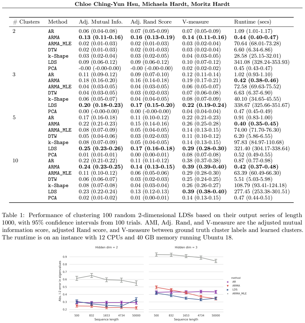
Because the method never attempts full system identification, it sidesteps the local-optima and runtime problems of likelihood-based LDS fitting while retaining comparable clustering quality on the reported experiments.

Reading between the lines

Editorial extensions of the paper, not claims the author makes directly.

A testable extension is overparameterization: when the assumed hidden dimension is larger than the true order, Theorem 4.1 predicts the extra eigenvalues appear as zeros in the AR polynomial; one could check whether spurious near-zero roots degrade clustering and whether explicitly truncating them helps.
The same AR-coefficient pipeline could serve as a feature map for anomaly detection or change-point analysis in physiological or financial records, where the dynamics shift and the eigenspectrum is the quantity of interest; that use is beyond the paper's clustering experiments.
For multi-site data collection with different device gains, the basis invariance of the spectrum suggests the fitted AR parameters can be pooled directly; a realistic test would be to record the same heart rhythm with two electrode configurations and confirm the estimated spectra agree.
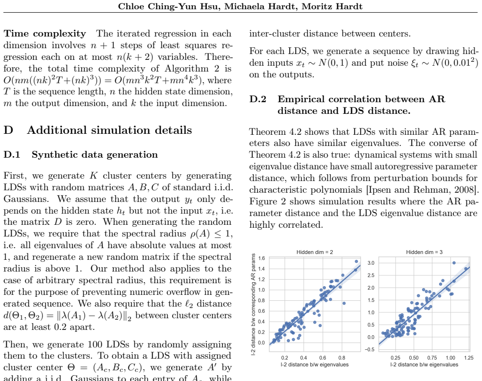
The converse perturbation bound mentioned in the appendix suggests the AR distance can serve as a proxy for eigenvalue distance in general; a sharp, finite-sample version of that converse would turn the clustering algorithm into a distance-based method with known distortion guarantees.

Share X Bluesky LinkedIn Reddit HN

Signed reviews

No signed human review yet.

Editorial analysis

A structured set of objections, weighed in public.

Desk editor's note, referee report, and a circularity audit.

Desk Editor's Note

read the letter

Katie,

Quick take: this paper deserves review. The core idea—estimate the eigenspectrum of an LDS from output alone via the AR parameters of its equivalent ARMA model, skipping full system identification—is sound and practical. The authors credit the classical LDS-ARMA equivalence (Åström–Wittenmark, Kailath) and build on it with something new: an explicit condition-number bound for simple eigenvalues via Vandermonde inversion, and a regularized iterated-regression estimator that is fast and works well. Clustering experiments on synthetic and ECG data are convincing, and the basis-invariance is a real plus when measurement procedures differ across sources.

The soft spots are real but local. The advertised O_p(T^{-1/2}) eigenvalue rate is only justified for simple spectra. Theorem 4.2 itself gives O(ε^{1/n}) in general and O(ε) for simple eigenvalues; with repeated eigenvalues the rate is strictly worse. The Introduction and Section 6.3 state the fast rate without qualification, and the experiments use random matrices, which have simple eigenvalues almost surely, so the faster rate is untested for repeated spectra. Second, Theorem 4.2 defines r_i as roots of 1 − φ̂_1 z − ... − φ̂_n z^n, which is the reciprocal lag polynomial; its roots are reciprocals of the eigenvalues, not the eigenvalues. As written, that theorem is literally false. The fix is easy—use the monic polynomial z^n − φ̂_1 z^{n−1} − ... − φ̂_n—and Appendix B already works with the monic polynomial, so this is a statement bug, not a proof bug. Still, it should be corrected. Third, the claim that adding regularization preserves O(T^{-1/2}) consistency is asserted without proof. Plausible, but it needs a citation or a proof. Finally, the regularization coefficient for synthetic data is unreported, and the ECG value (0.01) was chosen based on simulation. Disclose it and show sensitivity.

None of this sinks the central contribution. The method works, the theory is mostly right, and the writing is clear. I'd send this to a serious referee with a request to fix the reciprocal issue and qualify the convergence claims. For the time series/ML crowd, this is worth knowing.

Best

Referee Report

4 major / 4 minor

Summary. The paper proposes a method to estimate the eigenvalues of the state-transition matrix A of a linear dynamical system (LDS) from output time series alone, without full system identification. The theoretical core is a correspondence between LDSs and ARMA/ARMAX models: the autoregressive parameters of the output series recover the characteristic polynomial of A (Theorem 4.1), and small AR-parameter error implies small eigenvalue error, with a general O(epsilon^{1/n}) bound and an O(epsilon) bound under simplicity (Theorems 4.2 and 4.3). The authors combine this with the consistent iterated-regression estimator of Tsay and Tiao (1984), adding L2 regularization on the MA coefficients, to obtain a practical algorithm with an advertised O_p(T^{-1/2}) eigenvalue convergence rate. The method is applied to time series clustering, with experiments on synthetic LDS data and real ECG signals showing competitive clustering quality and much lower runtime than EM-based LDS baselines.

Significance. If the main claims hold, the paper makes a useful conceptual point: meaningful information about linear dynamics (the eigenspectrum) can be learned from outputs without solving the hard full-identification problem. The model equivalence is standard but the paper gives explicit perturbation bounds and a computationally simple algorithm with code. The clustering application is natural and the experiments are reasonable. However, the advertised convergence rate is only proven under a simplicity assumption, and one theorem statement contains a reciprocal-polynomial error; these are local but load-bearing issues that the authors should fix.

major comments (4)

[Theorem 4.2] The statement defines r_i as the roots of the polynomial 1 - phi_hat_1 z - ... - phi_hat_n z^n. This is the reciprocal lag polynomial, whose roots are the reciprocals of the eigenvalues (since the characteristic polynomial is lambda^n - phi_1 lambda^{n-1} - ... - phi_n). As written, the claim that these roots converge to the true eigenvalues is literally false. The monic polynomial z^n - phi_hat_1 z^{n-1} - ... - phi_hat_n should be used instead.
[Abstract, Section 1, Section 6.3] The paper repeatedly states that eigenvalues are estimated at rate O_p(T^{-1/2}) without qualification. Theorem 4.2 gives O(epsilon) only when all eigenvalues are simple; in the general case the rate is O(epsilon^{1/n}), which combined with Theorem 5.1 gives only O_p(T^{-1/(2n)}). The unqualified statements in the abstract, introduction, and Section 6.3 are therefore not supported by the theorems. The simplicity assumption should be stated wherever the O_p(T^{-1/2}) eigenvalue rate is claimed.
[Section 5, 'Convergence rate'] The claim that adding L2 regularization to the MA coefficients 'does not change the asymptotic property of the estimator' is asserted without proof or citation. Theorem 5.1 covers the unregularized iterated regression of Tsay and Tiao (1984), not Algorithm 1 as proposed. Since the paper's consistency and rate claims apply to the regularized algorithm, this gap needs to be filled (or the claim qualified).
[Theorem 4.1 and Appendix A.2] The theorem as stated claims that every output dimension of any LDS is ARMAX(n,n,n-1) with AR parameters recovering the characteristic polynomial. The proof in Appendix A.2 requires the additional assumption that there are no common factors in chi^dagger_A and Gamma (no pole-zero cancellation) to conclude that chi^dagger_A is the AR polynomial. Without this assumption the output series can be generated by a lower-order ARMA model and the full eigenspectrum of A is not recoverable from the AR parameters. This condition should be part of the theorem statement (and of Corollary 4.1), not only of the proof.

minor comments (4)

[Equation (3) and Definition B.1] The companion matrix is defined with one orientation in Definition B.1 and used with a different sign/orientation in the state-space construction in Equation (3) (C(-Phi)^T). This makes the simple-eigenvalue proof harder to follow; the conventions should be reconciled.
[Corollary 4.1] The 'if and only if' claim for LDSs of different dimensions relies on the no-cancellation premise; the paper should explicitly connect this to the assumption of Theorem 4.1.
[Section 5.1] The claim that multidimensional outputs share the same autoregressive parameters and that averaging per-channel estimates preserves the statistical rate is not justified; a sentence of explanation or a citation would be helpful.
[General] Figure 1 is referenced as showing eigenvalue estimation error, but the captioned figure content is not reproduced in the text I reviewed; the authors should ensure the figure is present and readable in the final version.

Circularity Check

0 steps flagged · score 0.0 of 10

No significant circularity: the eigenvalue estimates are derived from an external ARMA estimator applied to the output series, with no target eigenvalue entering the estimation procedure.

full rationale

The central derivation is self-contained and not circular. Theorem A.1 proves, from the LDS state equations (1) and the generalized-eigenvector lemma (Lemma A.2), that the output satisfies χ†_A(L)y_t = χ†_A(L)ξ_t + Γ(L)x_t, so the AR polynomial is the reciprocal characteristic polynomial of A; Theorem 4.1 then reads off the AR coefficients from χ_A. No eigenvalue of A is used as an input to the estimation procedure. The estimator in Algorithm 1 is the external iterated-regression method of Tsay and Tiao (1984), and its O_p(T^{-1/2}) consistency is quoted from that independent source; the paper's own contribution is the polynomial-root continuity argument (Theorem 4.2) connecting AR-coefficient error to eigenvalue error, which is a standard perturbation bound (Lemma B.1). The regularization strength α is a tuning constant and is not a fitted version of any target eigenvalue. The only self-citation (Hardt et al. 2018) appears as background in related work and does not carry any load-bearing step. The reciprocal-polynomial convention in Theorem 4.2 and the O(T^{-1/2}) rate in the repeated-eigenvalue case are correctness concerns, not instances of circular reasoning, and do not raise the circularity score.

Assumptions & free parameters 1 free parameters · 7 assumptions · 0 invented entities

The paper rests on standard LDS modeling assumptions, the classical LDS-ARMA correspondence, and external results from time series estimation and perturbation theory. The only fitted quantity is the regularization coefficient α, which affects practical performance but not the theoretical correctness.

free parameters (1)

regularization coefficient α = 0.01 (ECG); unreported (synthetic)
The L2-regularization strength on the moving-average coefficient estimates in Algorithm 1. Section 6.4 says the ECG value 0.01 was 'chosen based on our simulation results', but no value is reported for the synthetic experiments, which is a reproducibility gap.

assumptions (7)

domain assumption The LDS is observable: C, CA, CA^2, ..., CA^{n-1} are linearly independent.
Stated in Section 3.1; without it, the ARMA order reduces and the full eigenspectrum is not identifiable from the output.
domain assumption No pole-zero cancellation: no common factors in χ†_A(L) and Γ(L).
Assumed in the proof of Theorem A.1 (Appendix A.2) so that χ†_A is the AR polynomial; otherwise the AR parameters do not reveal all eigenvalues.
domain assumption The hidden state dimension n is known a priori.
Algorithm 1 takes n as input; the paper does not analyze model selection for unknown n.
domain assumption The noise in the LDS is diagonal Gaussian.
Stated in Section 3.1, used in the ARMA reduction for hidden inputs (Appendix A.3).
standard math Tsay and Tiao (1984) iterated regression provides a consistent estimator of AR parameters in ARMA models with rate O(T^{-1/2}).
Invoked in Section 5 and Theorem 5.1; no proof is given in this paper, but it is an external published result.
standard math The sum of ARMA processes remains an ARMA process (Granger and Morris 1976).
Used in Lemma A.1 to combine the hidden-input ARMA(n,n-1) process with measurement noise ARMA(0,0).
standard math Standard polynomial root perturbation bounds (Beauzamy; Lancaster et al.) apply.
Used in Theorem 4.2 and Lemma B.2 for the O(ε^{1/n}) and O(ε) eigenvalue convergence rates.

how reviews work

0 comments

Cite this review

Pith. "Pith review of Linear Dynamics: Clustering without identification." pith.science (2026). https://pith.science/paper/CPI3O4DG

@misc{pith2026190801039,
  author       = {Pith},
  title        = {Pith review of: Linear Dynamics: Clustering without identification},
  year         = {2026},
  howpublished = {\url{https://pith.science/paper/CPI3O4DG}},
  note         = {Machine review of arXiv:1908.01039}
}

read the original abstract

Linear dynamical systems are a fundamental and powerful parametric model class. However, identifying the parameters of a linear dynamical system is a venerable task, permitting provably efficient solutions only in special cases. This work shows that the eigenspectrum of unknown linear dynamics can be identified without full system identification. We analyze a computationally efficient and provably convergent algorithm to estimate the eigenvalues of the state-transition matrix in a linear dynamical system. When applied to time series clustering, our algorithm can efficiently cluster multi-dimensional time series with temporal offsets and varying lengths, under the assumption that the time series are generated from linear dynamical systems. Evaluating our algorithm on both synthetic data and real electrocardiogram (ECG) signals, we see improvements in clustering quality over existing baselines.

Figures

Figures reproduced from arXiv: 1908.01039 by the authors.

**Figure 1.** Absolute `2-error in eigenvalue estimation for 2-dimensional and 3-dimensional LDSs, with 95% confidence interval from 500 trials. Method AMI Adj. Rand Score V-measure ARMA 0.12 (0.10-0.13) 0.12 (0.11-0.14) 0.14 (0.12-0.16) AR 0.10 (0.09-0.12) 0.10 (0.09-0.12) 0.13 (0.11-0.14) PCA 0.04 (0.03-0.05) 0.02 (0.02-0.03) 0.07 (0.06-0.08) LDS 0.09 (0.07-0.10) 0.11 (0.10-0.13) 0.10 (0.09-0.11) k-Shape 0.08 (0.07-0.10) 0.09 (… view at source ↗

**Figure 2.** shows simulation results where the AR parameter distance and the LDS eigenvalue distance are highly correlated [PITH_FULL_IMAGE:figures/full_fig_p017_2.png] view at source ↗

Discussion (0). Continue with ORCID to comment.

Reference graph

Works this paper leans on

12 extracted references · 10 canonical work pages

[1]

[Afsari et al., 2012]Afsari, B., Chaudhry, R., Ravichandran, A., and Vidal, R. (2012). Group action induced distances for averaging and clustering linear dynamical systems with applications to the analysis of dynamic scenes. In 2012 IEEE Conference on Computer Vision and Pattern Recognition, pages 2208–2215. IEEE. [Åström and Wittenmark, 2013]Åström, K. J...

work page 2012
[3]

Theorem B.1

the explicit condition number bounds for the simple eigenvalue case. Theorem B.1. Suppose yt are the outputs from an n-dimensional latent linear dynamical system with pa- rameters Θ = (A,B,C,D ) and eigenvaluesλ1,··· ,λn. Let ˆΦ = ( ˆϕ1,··· , ˆϕn) be the estimated autoregressive parameters with error‖ˆΦ− Φ‖ =ϵ, and letr1,··· ,rn be the roots of the polyno...

work page 1999
[6]

Lemma B.2(Theorem 6 in [Lancaster et al., 2003])

It is known that regular splitting holds for any semi-simple eigenvalue even for non-Hermitian matrices. Lemma B.2(Theorem 6 in [Lancaster et al., 2003]). Let L(λ,ϵ ) be an analytic matrix function with semi- simple eigenvalueλ0 at ϵ = 0 of multiplicityM. Then there are exactlyM eigenvalues λi(ϵ) of L(λ,ϵ ) for which λi(ϵ)→λ0 as ϵ→ 0, and for these eigenv...

work page 2003
[7]

TheO(ϵ) convergence rate then follows from Lemma B.2 and Theorem 5.1, as the error on ARMAX parameter estimation can be seen as perturbation on the companion matrix

Since this LDS the same autoregressive parameters and hidden state dimension as the original LDS, by Corollary 4.1 the companion matrix has the same characteristic polynomial as the original LDS, and thus also has simple (and hence also semi-simple) eigenvalues. TheO(ϵ) convergence rate then follows from Lemma B.2 and Theorem 5.1, as the error on ARMAX pa...

work page 2003
[8]

Hence the outputsyt are generated by an ARMA(n,n) process as claimed in Theorem 4.1

= ARMA(n + 0, max(n + 0,n− 1 + 0)) = ARMA(n,n). Hence the outputsyt are generated by an ARMA(n,n) process as claimed in Theorem 4.1. It is easy to see in the proof of Lemma A.1 that the autoregressive parameters do not change when adding a white noise [Granger and Morris, 1976]. B Proof for eigenvalue approximation theorems Here we restate Theorem 4.2 and...

work page 1976
[12]

D.2 Empirical correlation between AR distance and LDS distance

and put noiseξt∼N(0, 0.012) on the outputs. D.2 Empirical correlation between AR distance and LDS distance. Theorem 4.2 shows that LDSs with similar AR param- eters also have similar eigenvalues. The converse of Theorem 4.2 is also true: dynamical systems with small eigenvaluedistancehavesmallautoregressiveparameter distance, which follows from perturbati...

work page 2008
[15]

[Hardt et al., 2018]Hardt, M., Ma, T., and Recht, B. (2018). Gradient descent learns linear dynamical systems. The Journal of Machine Learning Research, 19(1):1025–1068. [Hazan et al., 2018]Hazan, E., Lee, H., Singh, K., Zhang, C., and Zhang, Y. (2018). Spectral ﬁltering for general linear dynamical systems. InAdvances in Neural Information Processing Sys...

work page 2018
[61]

[Simchowitz et al., 2018]Simchowitz, M., Mania, H., Tu, S., Jordan, M

Scipy. [Simchowitz et al., 2018]Simchowitz, M., Mania, H., Tu, S., Jordan, M. I., and Recht, B. (2018). Learn- ing without mixing: Towards a sharp analysis of linear system identiﬁcation. arXiv preprint arXiv:1802.08334. [Smyth, 1997] Smyth, P. (1997). Clustering sequences with hidden markov models. InAdvances in neural information processing systems, pag...

arXiv 2018

Show all 12 references

[156]

[Kalman, 1960] Kalman, R

Prentice-Hall Englewood Cliﬀs, NJ. [Kalman, 1960] Kalman, R. E. (1960). A new approach to linear ﬁltering and prediction problems.Journal of basic Engineering, 82(1):35–45. [Kalpakis et al., 2001]Kalpakis, K., Gada, D., and Puttagunta, V. (2001). Distance measures for eﬀec- ti...

1960
[207]

X., Epps, J., and Bailey, J

[Vinh et al., 2010]Vinh, N. X., Epps, J., and Bailey, J. (2010). Information theoretic measures for cluster- ings comparison: Variants, properties, normalization and correction for chance.Journal of Machine Learn- ing Research, 11(Oct):2837–2854. [Vishwanathan et al., 2007]Vis...

2010
[295]

Y., Rajpurkar, P., Haghpanahi, M., Tison, G

[Hannun et al., 2019]Hannun, A. Y., Rajpurkar, P., Haghpanahi, M., Tison, G. H., Turakhia, M. P., Bourn, C., and Ng, A. Y. (2019). Cardiologist-level arrhythmia detection and classiﬁcation in ambula- tory electrocardiograms using a deep neural network. Nature Medicine,

2019
[6726]

[Chan and Vasconcelos, 2005]Chan, A. B. and Vas- concelos, N. (2005). Probabilistic kernels for the classiﬁcation of auto-regressive visual processes. In 2005 IEEE Computer Society Conference on Com- puter Vision and Pattern Recognition (CVPR’05), volume 1, pages 846–851. IEEE...

2005 arXiv

Pith tools

Reviewed August 14, 2026 · model on record in the stance chip above.

[1] [1]

[Afsari et al., 2012]Afsari, B., Chaudhry, R., Ravichandran, A., and Vidal, R. (2012). Group action induced distances for averaging and clustering linear dynamical systems with applications to the analysis of dynamic scenes. In 2012 IEEE Conference on Computer Vision and Pattern Recognition, pages 2208–2215. IEEE. [Åström and Wittenmark, 2013]Åström, K. J...

work page 2012

[2] [3]

Theorem B.1

the explicit condition number bounds for the simple eigenvalue case. Theorem B.1. Suppose yt are the outputs from an n-dimensional latent linear dynamical system with pa- rameters Θ = (A,B,C,D ) and eigenvaluesλ1,··· ,λn. Let ˆΦ = ( ˆϕ1,··· , ˆϕn) be the estimated autoregressive parameters with error‖ˆΦ− Φ‖ =ϵ, and letr1,··· ,rn be the roots of the polyno...

work page 1999

[3] [6]

Lemma B.2(Theorem 6 in [Lancaster et al., 2003])

It is known that regular splitting holds for any semi-simple eigenvalue even for non-Hermitian matrices. Lemma B.2(Theorem 6 in [Lancaster et al., 2003]). Let L(λ,ϵ ) be an analytic matrix function with semi- simple eigenvalueλ0 at ϵ = 0 of multiplicityM. Then there are exactlyM eigenvalues λi(ϵ) of L(λ,ϵ ) for which λi(ϵ)→λ0 as ϵ→ 0, and for these eigenv...

work page 2003

[4] [7]

TheO(ϵ) convergence rate then follows from Lemma B.2 and Theorem 5.1, as the error on ARMAX parameter estimation can be seen as perturbation on the companion matrix

Since this LDS the same autoregressive parameters and hidden state dimension as the original LDS, by Corollary 4.1 the companion matrix has the same characteristic polynomial as the original LDS, and thus also has simple (and hence also semi-simple) eigenvalues. TheO(ϵ) convergence rate then follows from Lemma B.2 and Theorem 5.1, as the error on ARMAX pa...

work page 2003

[5] [8]

Hence the outputsyt are generated by an ARMA(n,n) process as claimed in Theorem 4.1

= ARMA(n + 0, max(n + 0,n− 1 + 0)) = ARMA(n,n). Hence the outputsyt are generated by an ARMA(n,n) process as claimed in Theorem 4.1. It is easy to see in the proof of Lemma A.1 that the autoregressive parameters do not change when adding a white noise [Granger and Morris, 1976]. B Proof for eigenvalue approximation theorems Here we restate Theorem 4.2 and...

work page 1976

[6] [12]

D.2 Empirical correlation between AR distance and LDS distance

and put noiseξt∼N(0, 0.012) on the outputs. D.2 Empirical correlation between AR distance and LDS distance. Theorem 4.2 shows that LDSs with similar AR param- eters also have similar eigenvalues. The converse of Theorem 4.2 is also true: dynamical systems with small eigenvaluedistancehavesmallautoregressiveparameter distance, which follows from perturbati...

work page 2008

[7] [15]

[Hardt et al., 2018]Hardt, M., Ma, T., and Recht, B. (2018). Gradient descent learns linear dynamical systems. The Journal of Machine Learning Research, 19(1):1025–1068. [Hazan et al., 2018]Hazan, E., Lee, H., Singh, K., Zhang, C., and Zhang, Y. (2018). Spectral ﬁltering for general linear dynamical systems. InAdvances in Neural Information Processing Sys...

work page 2018

[8] [61]

[Simchowitz et al., 2018]Simchowitz, M., Mania, H., Tu, S., Jordan, M

Scipy. [Simchowitz et al., 2018]Simchowitz, M., Mania, H., Tu, S., Jordan, M. I., and Recht, B. (2018). Learn- ing without mixing: Towards a sharp analysis of linear system identiﬁcation. arXiv preprint arXiv:1802.08334. [Smyth, 1997] Smyth, P. (1997). Clustering sequences with hidden markov models. InAdvances in neural information processing systems, pag...

arXiv 2018