REVIEW 5 major objections 5 minor 2 references
Ensemble Neural Networks (ENN): A gradient-free stochastic method
T0 review · 5 major / 5 minor · reviewed 2026-08-14 · deepseek-v4-flash
Pith's one-line read The paper claims that neural networks can be trained with no gradient computations at all, by replacing the sensitivity matrix with covariances estimated from an ensemble of weight realizations, and that this yields uncertainty estimates…
desk verdict A legitimate new application of EnRML to neural network training, but the covariance-to-gradient approximation is asserted rather than validated and the real-data comparisons are thin. read the letter →
The pith
A machine-rendered reading of the paper's core claim, the machinery that carries it, and where it could break.
The reading
What carries the argument
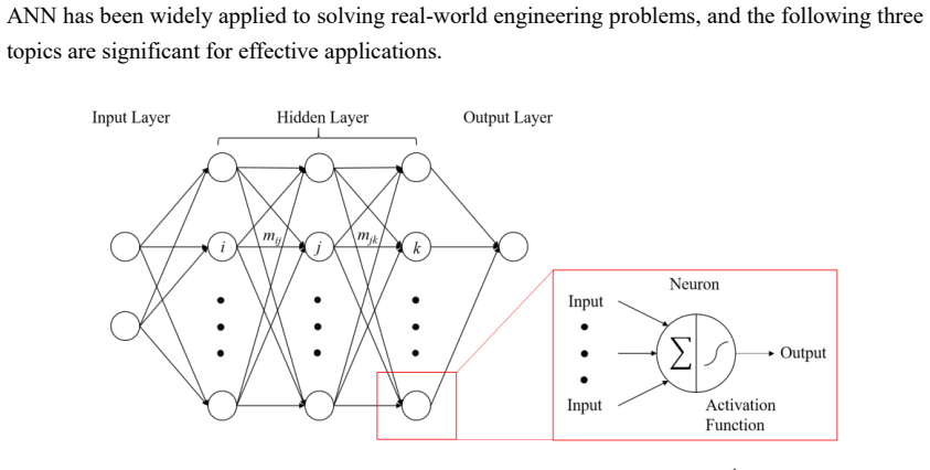
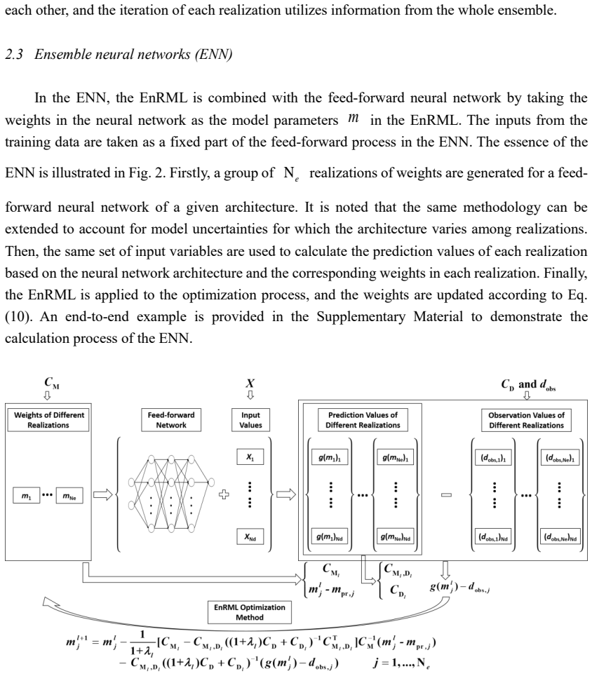
The load-bearing mechanism is the EnRML update of Eq. (10). EnRML is an ensemble-based inverse modeling algorithm that iteratively adjusts a set of parameter realizations to match observed data; here the parameters are the neural network weights and the forward map is the network's feed-forward computation. Instead of forming the sensitivity matrix $G$, it computes the cross-covariance $C_{M,D}^l$ between the current weight realizations and their predicted outputs, and the covariance $C_D^l$ of predicted outputs, and uses these in place of $G$ inside a Gauss-Newton step. A multiplier $\lambda$ regulates the step size: it grows when the ensemble's data mismatch worsens and shrinks when the mismatch improves, preventing over-updates early in training. The same ensemble of realizations thus does double duty: it provides the covariance statistics that drive optimization and, at convergence, provides the spread that gives predictive uncertainty intervals.
What would settle it
Take a regression problem with a deliberately nonlinear activation and initialize the ensemble with wide weight distributions; compute the sample cross-covariance $C_{M,D}$ and compare it against the product $C_M G^T$ using finite-difference gradients. If the relative discrepancy is large in early iterations and the ENN update fails to reduce test loss while gradient descent succeeds, the linearity assumption behind Eq. (10) is the point of failure.
Extended reading notes
Core claim
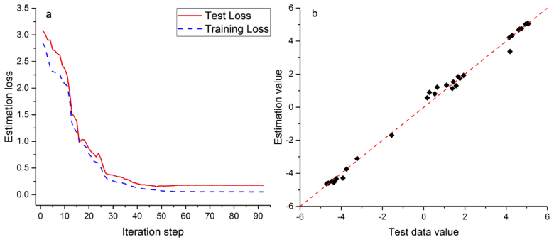
The discovery the paper argues for is that the Gauss-Newton update for a Bayesian neural-network objective can be made gradient-free by substituting ensemble covariances for the sensitivity matrix. Starting from the posterior $p(m|d_{\mathrm{obs}})\propto \exp[-O(m)]$, the objective $O(m)=\frac{1}{2}(m-m_{pr})^T C_M^{-1}(m-m_{pr})+\frac{1}{2}(g(m)-d_{\mathrm{obs}})^T C_D^{-1}(g(m)-d_{\mathrm{obs}})$ is minimized by repeated application of Eq. (10), in which $C_{M,D}^l$ (cross-covariance between weights and predicted outputs) and $C_D^l$ (covariance of predicted outputs) replace $G$. The justification is the first-order Taylor approximation $C_{M,D}=C_M G^T$, $C_D=G C_M G^T$, with residual terms neglected. The resulting update moves every realization toward its own perturbed observation, and the spread of the converged ensemble acts as the posterior uncertainty. The paper reports that this scheme converges on a synthetic problem with 70 training points and 93 weights, and that it achieves lower loss than three Bayesian neural network baselines across four real-world datasets.
Load-bearing premise
The method assumes the network's outputs are nearly linear in the weights across the ensemble's spread, so the sample covariance between weights and outputs equals the weight covariance times the gradient; if that linearity fails, the covariance proxy points the update in the wrong direction and convergence is not guaranteed.
Editorial extensions
If this is right
- Because no derivative of the network output is ever needed, the ENN update is compatible with neuron models and loss functions that are not differentiable, including biophysical neuron models and discrete evaluation metrics.
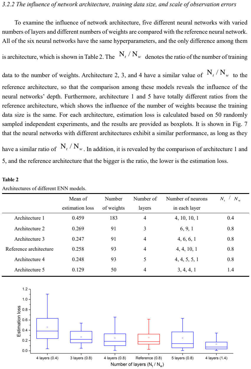
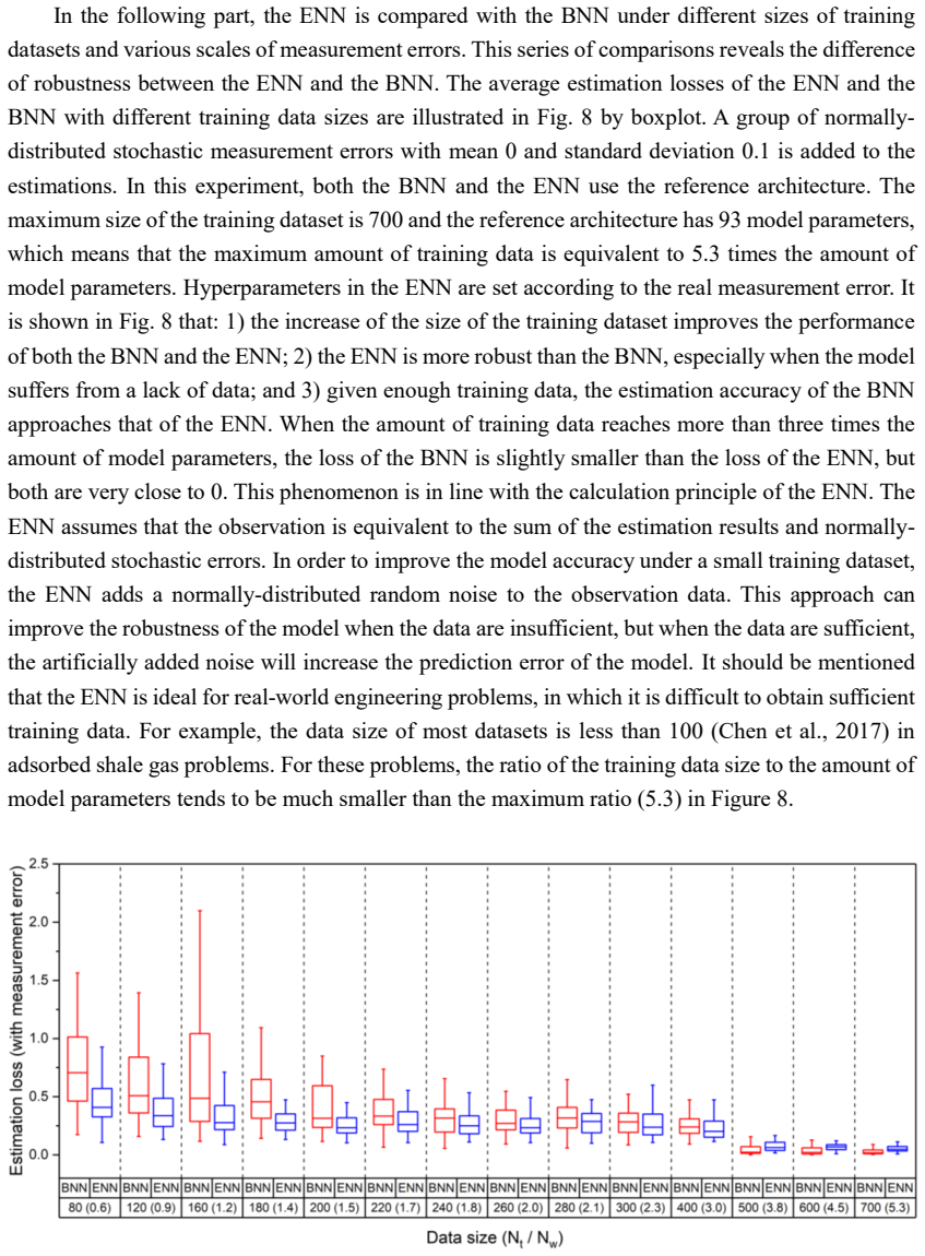
- The ensemble construction acts as implicit data augmentation, so ENN can train networks with more weights than training examples; the paper shows convergence with 70 training points and 93 weights and lower loss than BNN when data-to-weight ratios are small.
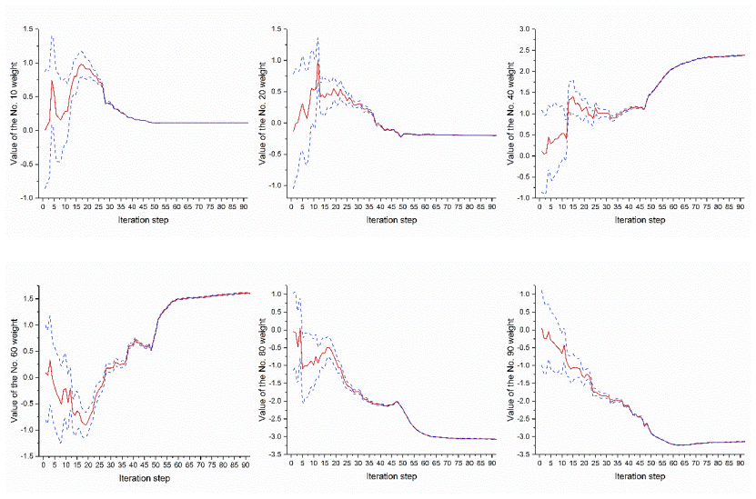
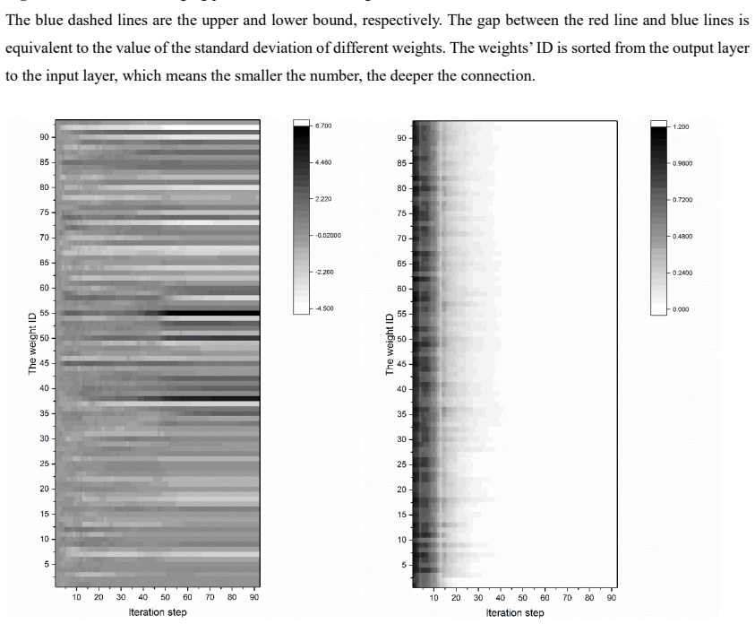
- Uncertainty quantification is a by-product of the optimization: the distribution of converged weight realizations directly supplies posterior predictive intervals, without a separate inference pass.
- With abundant training data the benefit shrinks: the paper observes that the BNN's loss approaches the ENN's as data grow, and a plain fully connected network can beat both when data are plentiful, so the practical advantage is concentrated in the small-data, uncertainty-requiring, gradient-free regime.
- Since the forward pass is unchanged, the same EnRML step can replace gradient descent in other architectures, including CNNs and RNNs, whenever their forward computations are well defined.
Reading between the lines
- A testable extension the paper does not run is to vary the ensemble size systematically; one would expect a bias-variance trade-off in the covariance proxy, with too few realizations making the update noisy and too many adding little.
- The covariance proxy suggests a direct link to natural-gradient and ensemble Kalman methods; if the approximation holds, any ensemble smoother could serve as a generic neural optimizer, not only EnRML.
- The paper compares only with traditional BNN; a fairer modern benchmark would include scalable approximate inference, and the distinctive claim of being gradient-free would survive even if the accuracy margin does not.
Signed reviews
Editorial analysis
A structured set of objections, weighed in public.
Referee Report
Summary. The paper proposes Ensemble Neural Networks (ENN), a training method for neural networks that replaces gradient-based backpropagation with an ensemble covariance update derived from the ensemble randomized maximum likelihood (EnRML) algorithm used in petroleum history matching. An ensemble of weight realizations is maintained; at each iteration the method computes cross-covariances between weights and predictions and the covariance of predictions, then updates all realizations through Eq. (10). The method is presented as gradient-free, Bayesian, naturally providing uncertainty quantification, and robust to small training data because the ensemble is said to enlarge the training set. Experiments include a one-dimensional toy regression, a synthetic 'ideal' regression problem, and four real-world datasets (three UCI plus one reservoir-simulation dataset), with comparisons against fully connected networks and three Bayesian neural network (BNN) variants.
Significance. If the central claims hold, the paper would offer a novel training paradigm for neural networks in small-data engineering settings, with built-in uncertainty estimates and no gradient computation. The connection between ensemble Kalman-filter-type methods and neural network training is timely and potentially valuable. The derivation is grounded in a mature inverse-modeling literature, and the supplementary material contains a hand-worked end-to-end example, which is a genuine reproducibility aid. The synthetic experiments in Section 3.2 use 50 independent runs and boxplots, which is good practice. However, the load-bearing covariance-to-gradient substitution is only heuristically justified, and the real-world experiments lack statistical rigor and adequate baseline specification.
major comments (5)
- [Section 2.2, Eq. (9) and Appendix D] The covariance-to-gradient substitution in Eq. (9) is the load-bearing step that converts the Gauss-Newton update (8) into the derivative-free update (10). Appendix D derives it by dropping all terms involving e_j - e_bar in Eqs. (D.6) and (D.7), justified by asserting that the first-order Taylor residual is small. For a ReLU network with weights initialized from a standard normal distribution, as in the Supplementary Material, the ensemble members at early iterations generically lie in different linear regions of the piecewise-linear map g(m), so a single sensitivity matrix G evaluated at the ensemble mean does not make the residual small; the neglected cross-terms can be of the same order as the retained covariance terms. Consequently the update direction in Eq. (10) need not approximate the direction of Eq. (8), and there is no guarantee that the objective (3) decreases. The paper contains no diagnostic measuring the approximation error on the architectures tested and no convergence proof. This is a central gap for the 'gradient-free' claim.
- [Section 1 and Section 4] The paper motivates gradient-free training by citing Hodgkin-Huxley neuron models and non-differentiable losses such as BLEU, and the Discussion repeats that the ENN is suitable for these settings. However, the only derivation connecting covariances to the update direction is the first-order Taylor expansion in Appendix D, which presupposes that g(m) is differentiable with respect to m. For non-differentiable neuron models or losses, the substitution in Eq. (9) has no theoretical basis, and no experiment with such models or losses is reported. The claim that the ENN 'enables the use of complicated neuron models and loss functions' is therefore not supported.
- [Section 3.3, Table 3] Table 3 reports average estimation losses for the real-world datasets without error bars, number of trials, or the train/test splitting protocol; it is not stated whether each entry is a single run or an average over many. The BNN baselines are not adequately specified: the prior variance, learning rate, number of iterations, and the validation procedure for BNN-Val are not given, so the reader cannot assess whether the comparison is favorable to the ENN by construction. No code is provided, which further limits reproducibility. As a result, the abstract's claim that 'the ENN performs much better than the traditional Bayesian neural networks' is not statistically established by the real-world experiments.
- [Section 2.3 and Section 4] The paper repeatedly attributes the small-data robustness of the ENN to the ensemble 'enlarging the training dataset' through duplication with random disturbance. This is only a heuristic: all realizations use the same input vectors and differ only in perturbed targets and initial weights, so no new information about the input-output mapping is introduced. The claimed mechanism is not quantified (e.g., no effective sample size or bias-variance analysis), and an alternative explanation is the regularizing prior term in Eq. (3). The authors should either provide a formal argument for this mechanism or temper the claim.
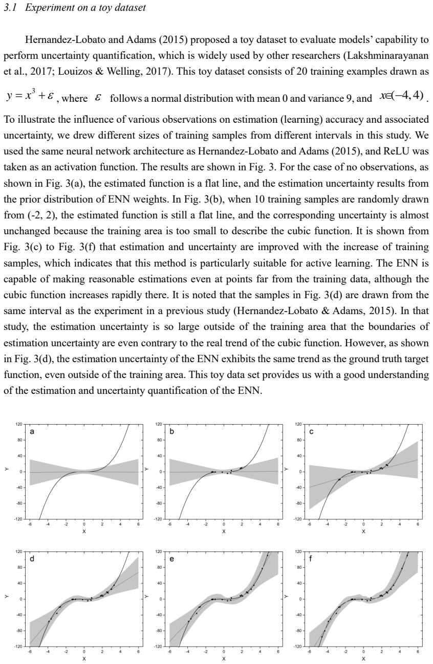
- [Section 3.1] The toy experiment demonstrates uncertainty bands qualitatively, but the paper does not quantitatively assess the quality of the uncertainty estimates (e.g., empirical coverage of the stated credible intervals, or sharpness of the predictive distributions). Given that uncertainty quantification is one of the primary advertised advantages of the ENN, the absence of any calibration metric leaves this claim unverified.
minor comments (5)
- [Appendix C] The text says 'the two equivalent equations in Eq. (6) and Eq. (7)' but the identities being derived are Eq. (5) and Eq. (6) of Section 2.2; the cross-references should be corrected.
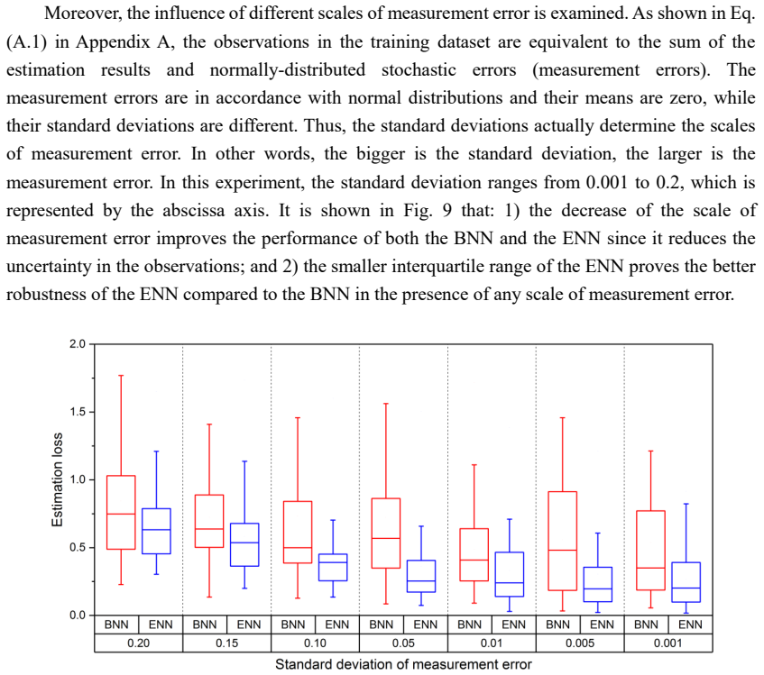
- [Section 3 and Supplementary Material] The loss metric used in Table 3 and Figures 7-9 is not defined in the main text; the supplementary material defines an absolute-error loss in Eq. (S.1), but it is unclear whether the real-world results use the same normalization.
- [Figure 3] The caption states that the gray area corresponds to three standard deviations, but the text does not specify whether this is the predictive uncertainty or the parameter uncertainty; this distinction is important for the uncertainty-quantification claims.
- [Appendix B] The values of the lower bound of lambda (0.005) and the factor gamma (10) are stated as fixed, but no sensitivity analysis is provided, so the reader cannot judge how the results depend on these choices.
- [Section 4] The claim that the ENN is 'simpler' than the BNN is not quantified; no runtime, memory, or iteration-count comparisons are reported.
Circularity Check
No significant circularity; the covariance update is an approximation, not a re-labeled fit, and comparisons are on held-out data.
full rationale
The derivation chain is explicit: Bayesian posterior (Eq. 2) implies the objective (Eq. 3); Gauss-Newton gives Eq. (4), reformulated to Eq. (8); then Eq. (9) substitutes covariance and cross-covariance for the sensitivity matrix, yielding the ensemble update Eq. (10). The only step that could resemble circularity is Eq. (9), but Appendix D derives it from a first-order Taylor expansion, C_M,D ≈ C_M G^T and C_D ≈ G C_M G^T, and explicitly discards the residual terms e_j - e_bar. This is an approximation with a stated linearity premise, not a definitional equivalence: C_M,D and C_D are computed from forward passes of the current ensemble, not from the target values used in the loss. No test-set quantity appears in the update; d_obs,j is a noise-perturbed copy of training targets, and C_D and C_M are prior hyperparameters. The reported losses are computed on held-out test data, including the 30-point test set in the ideal experiment and the external UCI and PRES-2D benchmarks, so no fitted parameter is being rediscovered as a prediction. The self-citations to Chen and Oliver (2010, 2013) and Zhang (2001) concern the EnRML machinery, but the covariance substitution used here is re-derived in Appendix D rather than imported as an unexamined uniqueness result. The statement that the ensemble enlarges the training data is a heuristic interpretation of noise-perturbed realizations, not a circular justification of the experimental outcomes. Overall, the central claim is an approximate, derivative-free update rule that is tested against independent baselines; no load-bearing step reduces by construction to its own inputs.
Assumptions & free parameters
free parameters (3)
- lambda lower bound and gamma =
0.005 and 10
- ensemble size Ne =
100
- observation noise standard deviation =
0.002 (default)
assumptions (4)
- domain assumption Observation model: d_obs = g(m) + epsilon with epsilon ~ N(0, C_D)
- domain assumption First-order Taylor expansion of g(m_j) around the ensemble mean with negligible residual error
- domain assumption Prior on weights is Gaussian with known mean m_pr and covariance C_M
- standard math Gauss-Newton Hessian ignores second derivatives of g(m)
Cite this review
Pith. "Pith review of Ensemble Neural Networks (ENN): A gradient-free stochastic method." pith.science (2026). https://pith.science/paper/LBU3KV5J
@misc{pith2026190801113,
  author       = {Pith},
  title        = {Pith review of: Ensemble Neural Networks (ENN): A gradient-free stochastic method},
  year         = {2026},
  howpublished = {\url{https://pith.science/paper/LBU3KV5J}},
  note         = {Machine review of arXiv:1908.01113}
}
read the original abstract
In this study, an efficient stochastic gradient-free method, the ensemble neural networks (ENN), is developed. In the ENN, the optimization process relies on covariance matrices rather than derivatives. The covariance matrices are calculated by the ensemble randomized maximum likelihood algorithm (EnRML), which is an inverse modeling method. The ENN is able to simultaneously provide estimations and perform uncertainty quantification since it is built under the Bayesian framework. The ENN is also robust to small training data size because the ensemble of stochastic realizations essentially enlarges the training dataset. This constitutes a desirable characteristic, especially for real-world engineering applications. In addition, the ENN does not require the calculation of gradients, which enables the use of complicated neuron models and loss functions in neural networks. We experimentally demonstrate benefits of the proposed model, in particular showing that the ENN performs much better than the traditional Bayesian neural networks (BNN). The EnRML in ENN is a substitution of gradient-based optimization algorithms, which means that it can be directly combined with the feed-forward process in other existing (deep) neural networks, such as convolutional neural networks (CNN) and recurrent neural networks (RNN), broadening future applications of the ENN.
Figures
Figures from the paper (6 more)
Reference graph
Works this paper leans on
-
[1]
Acharya, U. R., Oh, S. L., Hagiwara, Y ., Tan, J. H., & Adeli, H. (2018). Deep convolutional neural network for the automated detection and diagnosis of seizure using EEG signals. Computers in Biology and Medicine, 100, 270-278. Bertsekas, D. P. (1999). Nonlinear programming (pp. 1-60). Belmont: Athena Scientific. Bishop, C. (2007). Pattern recognition an...
work page 2018
-
[1998]
The 1998 IEEE International Joint Conference on (V ol
IEEE World Congress on Computational Intelligence. The 1998 IEEE International Joint Conference on (V ol. 1, pp. 753-756). IEEE. Kaya, H., Tüfekci, P., & Gürgen, F. S. (2012, March). Local and global learning methods for predicting power of a combined gas & steam turbine. In Proceedings of the International Conference on Emerging Trends in Computer and El...
arXiv 2018
Reviewed August 14, 2026 · model on record in the stance chip above.
Discussion (0). Continue with ORCID to comment.