REVIEW 4 major objections 5 minor 62 references
Learning Guided Convolutional Network for Depth Completion
T0 review · 4 major / 5 minor · reviewed 2026-08-14 · deepseek-v4-flash
Pith's one-line read Learning image-conditioned, spatially-variant kernels yields state-of-the-art depth completion on NYUv2 and KITTI.
desk verdict Solid, benchmark-driven depth completion paper with a genuinely useful memory-saving guided convolution; KITTI claims credible, NYUv2 numbers rest on the field's questionable inpainted ground truth. read the letter →
The pith
A machine-rendered reading of the paper's core claim, the machinery that carries it, and where it could break.
The reading
What carries the argument
The guided convolution module: a kernel-generating layer (KGL) produces a full set of spatially-variant weights from RGB features, then these weights are applied to depth features. To control memory, the paper factorizes the operation into a channel-wise spatially-variant convolution (per-channel $K \times K$ kernels) followed by a $1 \times 1$ cross-channel convolution whose weights are generated from a globally pooled image feature. This reduces per-pixel complexity from $O(M \cdot K^2)$ to $O(M + K^2)$ and memory by a factor close to $\frac{1}{N} + \frac{1}{K^2 \cdot H \cdot B}$, enabling fusion at multiple encoder stages.
What would settle it
Measure the method's edge-region error separately using high-quality dense depth from a different sensor (e.g., active stereo or structured-light scan) on a subset of KITTI/NYUv2 scenes. If the guided kernels' advantage over concatenation disappears or reverses on those true edge pixels, the reported gains are largely an artifact of smoothed or sparse supervision.
Extended reading notes
Core claim
The central claim is that feature fusion for depth completion should be guided by spatially-variant, image-dependent kernels rather than naive concatenation or addition. The paper argues that a network-generated kernel, conditioned on the RGB guidance image, can align depth features with object boundaries and scene content, and that the proposed factorization makes multi-stage fusion practical. The evidence is benchmark results: lower RMSE than existing published methods on the KITTI test set (736.24 mm versus 758.38 for DeepLiDAR) and the best RMSE on NYUv2 with both 200 and 500 samples.
Load-bearing premise
The evaluation assumes the ground-truth depth used for training and testing is accurate and representative, but the NYUv2 depth maps are produced by colorization inpainting that smooths edges, and the KITTI ground truth is semi-dense registered LiDAR; if these labels are biased, the reported gains may not transfer to true dense depth.
Editorial extensions
If this is right
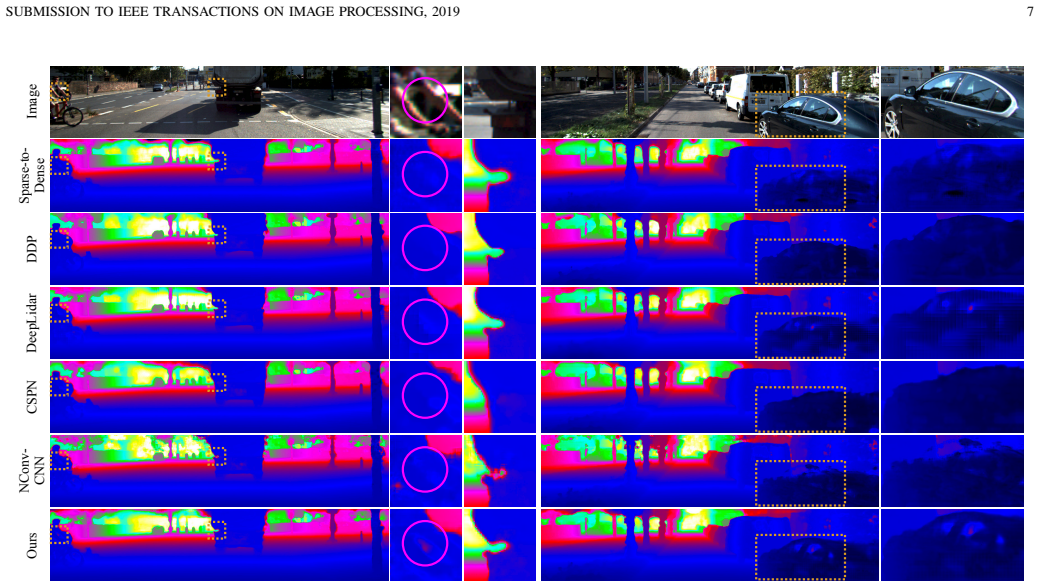
- On the KITTI test set, the method achieves RMSE 736.24 mm, better than DeepLiDAR (758.38), CSPN (1019.64), Sparse-to-Dense (814.73), DDP (832.94), NConv-CNN (829.98), and RGB-certainty (772.87).
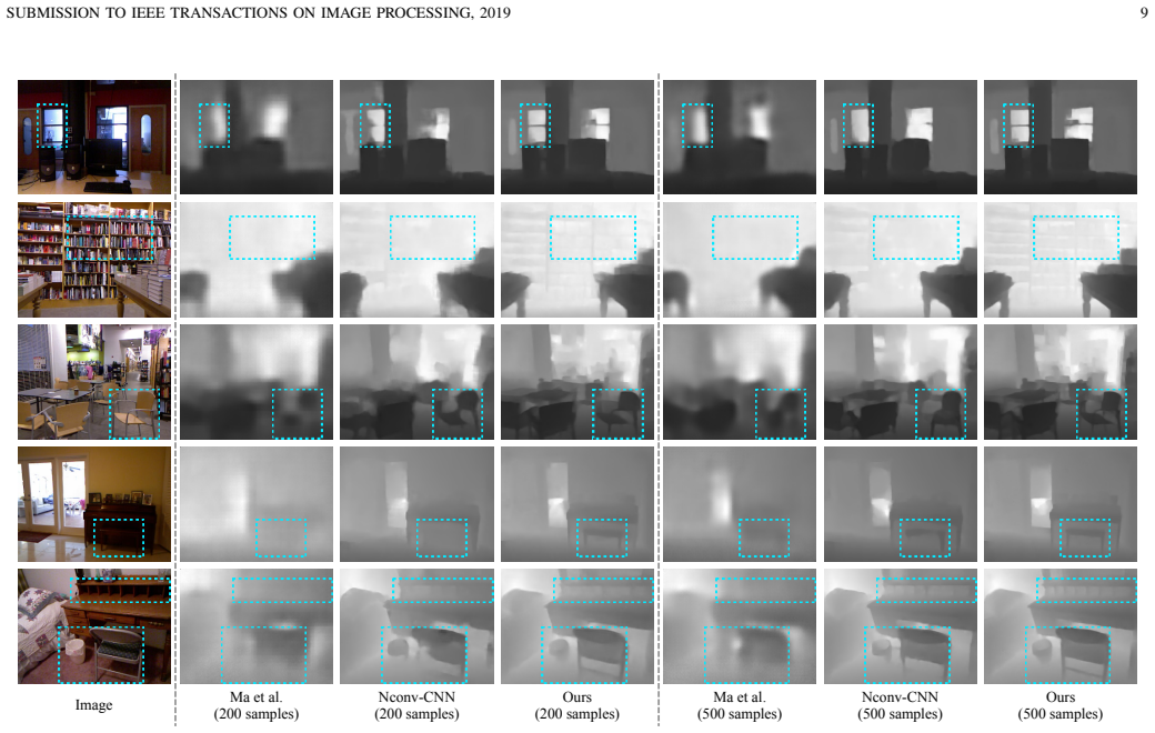
- On NYUv2, it reaches RMSE 0.101 with 500 samples and 0.142 with 200 samples, improving over all compared methods on all five metrics.
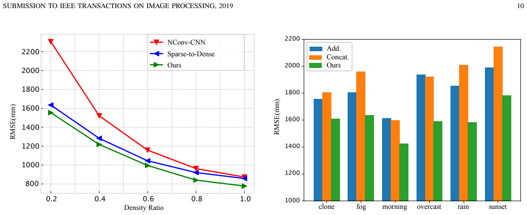
- Ablation studies show that replacing guided convolution with addition raises RMSE by 31.59 mm on the KITTI validation set, and concatenation raises it by 24.35 mm, so the guided module itself, not the network backbone, drives the gain.
- Fusing GuideNet decoder features into DepthNet encoder features in multiple stages outperforms early or late fusion, and keeping only the first or last guided stage underperforms multi-stage guidance.
- The model generalizes across LiDAR densities, lighting and weather conditions in Virtual KITTI, and from NYUv2 to SUN RGBD datasets with a different sensor.
Reading between the lines
- An untested consequence is that the same factorization should transfer to other tasks with heterogeneous inputs, such as RGB-guided semantic segmentation of sparse point clouds or image-guided upsampling of low-resolution depth, where spatially-variant fusion is currently done by concatenation.
- Because the generated kernels are conditioned purely on RGB features, the method implicitly learns to associate depth discontinuities with image edges; a small image-domain adversarial perturbation could therefore flip the kernels and corrupt the completed depth, a concern for safety-critical deployment.
- The reported memory reduction suggests the guided convolution could be applied at higher resolutions or with more fusion stages than the paper explores; testing on higher-resolution inputs is a natural extension.
- The method's robustness to point density implies it could adapt to cheaper, sparser sensors such as 16-line LiDAR with modest performance drop, but this is not directly tested on real 16-line data.
Editorial analysis
A structured set of objections, weighed in public.
Referee Report
Summary. The paper proposes a depth-completion network in which a "GuideNet" generates content-dependent, spatially-variant convolution kernels from an RGB image, and these kernels are applied to sparse depth features inside a "DepthNet." To make the scheme practical, the guided convolution is factorized into a spatially-variant channel-wise stage and a spatially-invariant cross-channel 1x1 stage, with a memory-reduction analysis in Eq. (8). The network fuses GuideNet decoder features into DepthNet encoder features at multiple scales. Experiments report rank 1 on the KITTI depth-completion leaderboard at the time of submission, state-of-the-art results on NYUv2, plus ablations and generalization tests under different point densities, lighting/weather conditions, and cross-dataset settings.
Significance. If the empirical claims hold, this is a solid contribution to depth completion and to multi-modal feature fusion more broadly. The factorization analysis in Eq. (8) is mathematically correct and the memory saving is substantial. The KITTI claim is especially strong because it is evaluated by the external test server, and the paper includes careful ablations of fusion position and multi-stage guidance. The generalization experiments across point density, lighting/weather, and datasets are a useful addition. The main weaknesses are empirical: the NYUv2 evaluation uses colorization-inpainted ground truth, no uncertainty quantification is provided for the small performance gaps, and some comparison rows are taken from prior papers while others are re-run by the authors.
major comments (4)
- [Section IV-A, Eq. (9), Table III] The NYUv2 ground truth is depth in-painted with the official colorization toolbox, and the loss in Eq. (9) treats these interpolated values as valid targets. Since the central mechanism of the paper is RGB-guided, spatially-variant kernel generation, the reported NYUv2 advantage over DeepLiDAR and CSPN could partly reflect fitting smooth colorization structure rather than measured Kinect geometry. Please add an evaluation on raw valid Kinect pixels (or on the measured depth before inpainting) and explicitly quantify how much of the improvement survives under that more conservative reference.
- [Section IV-D and Table III] All reported numbers are from a single training run, and several key gaps are small (e.g., NYUv2 RMSE 0.101 vs. 0.115 for DeepLiDAR and 0.117 for CSPN in Table III). Without error bars or multiple-seed runs, the claim of outperforming prior methods on NYUv2 is not statistically grounded. Please report mean and standard deviation over at least three runs for the main comparisons and ablations, or justify why a single run is sufficient for these conclusions.
- [Section IV-E and Table III] Table III mixes numbers quoted from previous papers with numbers the authors obtained by running released implementations. To make the comparison meaningful, the paper must state explicitly that identical preprocessing, sparse-sample generation, cropping, padding, and evaluation masks are used for all rows, and must list which rows were re-run and which were transcribed from prior publications. This is especially important for the 200-sample setting, where missing rows for CSPN and DeepLiDAR make the sentence "outperforms all other methods in both settings" unsupported as written.
- [Section III-C, Eqs. (5)-(8)] The statement that the factorization reduces the computational complexity of D_{p,n} from O(M*K^2) to O(M+K^2) is only valid if the channel-wise stage of Eq. (6) is computed once and amortized across all N output channels. In a from-scratch computation of a single output element, Eq. (6) still costs O(M*K^2). Please state the amortization assumption explicitly and report the actual total FLOPs ratio, since the paper's abstract claims a reduction in computation as well as memory.
minor comments (5)
- [Throughout] There are several typographical errors, including "naïvely" in the abstract, "Equqation (2)" in Section III-C, "datset" in Section IV-A, and "futher" in Section IV-A; these should be corrected.
- [Figure 1 and Section III] The naming is inconsistent between "GuideNet" and "GuidedNet" across the text and figure legend; please unify the terminology.
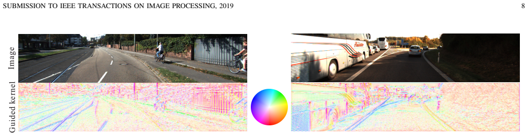
- [Section IV-C] The kernel visualization in Figure 4 is acknowledged as "extremely rough," but the accompanying claim that it "confirms" the kernels are content-dependent is stronger than the evidence warrants; please soften this to "is consistent with" or add a quantitative evaluation of kernel alignment with image boundaries.
- [Section IV-E and Table III] The 200-sample block of Table III does not include CSPN or DeepLiDAR, even though the text says the method outperforms all other methods under both settings; please add those results or qualify the claim.
- [Abstract and Table I] The claim "ranks 1st on the KITTI depth completion benchmark" is time-dependent; please state the submission date explicitly in the paper and note that leaderboard rankings can change.
Circularity Check
No significant circularity: the central claims are empirical benchmark results evaluated against external datasets, and the architecture is trained end-to-end without re-stating fitted parameters as predictions.
full rationale
The paper's central claim is an empirical benchmark result: it reports RMSE and related metrics on the KITTI leaderboard and on the NYUv2 dataset, both of which are external evaluation protocols. The proposed guided convolution module generates content-dependent, spatially-variant kernels from the guidance image and applies them to depth features; the kernel weights are outputs of learned network layers (the Kernel-Generating Layer), not fitted parameters that are later renamed as predictions. The depth completion loss in Eq. (9) measures the prediction against ground-truth depth, and no quantity that is used as an input to the method is also presented as a derived result. The ablation studies compare architectural variants under the same training and evaluation settings, and the comparison numbers for prior methods come from their published papers or released implementations. The reliance on guided image filtering and dynamic filtering is as inspiration, not as an unexamined self-citation that forces the conclusion. The use of colorization-inpainted NYUv2 ground truth is a property of the benchmark shared by all compared methods; it concerns the validity of the evaluation reference, not a circular derivation. No step in the paper reduces, by construction or self-citation, to its own inputs.
Assumptions & free parameters
free parameters (3)
- Kernel size K of guided convolution =
3
- Fusion scheme (decoder-to-encoder) =
D-E
- Channel widths M,N in fusion stages =
128 (example used in memory analysis)
assumptions (5)
- domain assumption The KITTI ground-truth depth (semi-dense registered LiDAR) is reliable enough for training and evaluation.
- domain assumption The NYUv2 depth maps are valid after inpainting with the official colorization toolbox.
- domain assumption Content-dependent spatially-variant kernels generated from RGB features can be applied to sparse depth features at multiple stages without losing essential information.
- domain assumption RGB and LiDAR inputs are accurately calibrated and synchronized.
- domain assumption The factorization into channel-wise convolution followed by 1x1 cross-channel convolution preserves enough capacity for the task.
Cite this review
Pith. "Pith review of Learning Guided Convolutional Network for Depth Completion." pith.science (2026). https://pith.science/paper/O44MBHOP
@misc{pith2026190801238,
  author       = {Pith},
  title        = {Pith review of: Learning Guided Convolutional Network for Depth Completion},
  year         = {2026},
  howpublished = {\url{https://pith.science/paper/O44MBHOP}},
  note         = {Machine review of arXiv:1908.01238}
}
read the original abstract
Dense depth perception is critical for autonomous driving and other robotics applications. However, modern LiDAR sensors only provide sparse depth measurement. It is thus necessary to complete the sparse LiDAR data, where a synchronized guidance RGB image is often used to facilitate this completion. Many neural networks have been designed for this task. However, they often na\"{\i}vely fuse the LiDAR data and RGB image information by performing feature concatenation or element-wise addition. Inspired by the guided image filtering, we design a novel guided network to predict kernel weights from the guidance image. These predicted kernels are then applied to extract the depth image features. In this way, our network generates content-dependent and spatially-variant kernels for multi-modal feature fusion. Dynamically generated spatially-variant kernels could lead to prohibitive GPU memory consumption and computation overhead. We further design a convolution factorization to reduce computation and memory consumption. The GPU memory reduction makes it possible for feature fusion to work in multi-stage scheme. We conduct comprehensive experiments to verify our method on real-world outdoor, indoor and synthetic datasets. Our method produces strong results. It outperforms state-of-the-art methods on the NYUv2 dataset and ranks 1st on the KITTI depth completion benchmark at the time of submission. It also presents strong generalization capability under different 3D point densities, various lighting and weather conditions as well as cross-dataset evaluations. The code will be released for reproduction.
Figures


Figures from the paper (4 more)

Reference graph
Works this paper leans on
-
[1]
Stereo processing by semiglobal matching and mu- tual information,
H. Hirschmuller, “Stereo processing by semiglobal matching and mu- tual information,” IEEE Transactions on pattern analysis and machine intelligence (TPAMI), vol. 30, no. 2, pp. 328–341, 2008
work page 2008
-
[2]
Evaluation of stereo matching costs on images with radiometric differences,
H. Hirschmuller and D. Scharstein, “Evaluation of stereo matching costs on images with radiometric differences,” IEEE transactions on pattern analysis and machine intelligence (TPAMI) , vol. 31, no. 9, pp. 1582– 1599, 2009
work page 2009
-
[3]
Computing the stereo matching cost with a convolutional neural network,
J. Zbontar and Y . LeCun, “Computing the stereo matching cost with a convolutional neural network,” in IEEE conference on computer vision and pattern recognition (CVPR) , 2015, pp. 1592–1599
work page 2015
-
[4]
Efficient deep learning for stereo matching,
W. Luo, A. G. Schwing, and R. Urtasun, “Efficient deep learning for stereo matching,” in IEEE Conference on Computer Vision and Pattern Recognition (CVPR) , 2016, pp. 5695–5703
work page 2016
-
[5]
J. Uhrig, N. Schneider, L. Schneider, U. Franke, T. Brox, and A. Geiger, “Sparsity invariant cnns,” in International Conference on 3D Vision (3DV). IEEE, 2017, pp. 11–20
work page 2017
-
[6]
J. Qiu, Z. Cui, Y . Zhang, X. Zhang, S. Liu, B. Zeng, and M. Pollefeys, “Deeplidar: Deep surface normal guided depth prediction for outdoor scene from sparse lidar data and single color image,” arXiv preprint arXiv:1812.00488, 2018
work page Pith review arXiv 2018
-
[7]
Self-supervised sparse- to-dense: Self-supervised depth completion from lidar and monocular camera,
F. Ma, G. V . Cavalheiro, and S. Karaman, “Self-supervised sparse- to-dense: Self-supervised depth completion from lidar and monocular camera,” arXiv preprint arXiv:1807.00275 , 2018
arXiv 2018
-
[8]
Dense disparity maps from sparse disparity measurements,
S. Hawe, M. Kleinsteuber, and K. Diepold, “Dense disparity maps from sparse disparity measurements,” in IEEE International Conference on Computer Vision (ICCV) , 2011, pp. 2126–2133
work page 2011
Show all 62 references
-
[9]
Depth reconstruction from sparse samples: Representation, algorithm, and sampling,
L.-K. Liu, S. H. Chan, and T. Q. Nguyen, “Depth reconstruction from sparse samples: Representation, algorithm, and sampling,” IEEE Transactions on Image Processing (TIP) , vol. 24, no. 6, pp. 1983–1996, 2015
1983
-
[10]
In defense of classical image processing: Fast depth completion on the cpu,
J. Ku, A. Harakeh, and S. L. Waslander, “In defense of classical image processing: Fast depth completion on the cpu,” in 15th Conference on Computer and Robot Vision (CRV) , 2018, pp. 16–22
2018
-
[11]
Sparse and dense data with cnns: Depth completion and semantic segmentation,
M. Jaritz, R. De Charette, E. Wirbel, X. Perrotton, and F. Nashashibi, “Sparse and dense data with cnns: Depth completion and semantic segmentation,” in International Conference on 3D Vision (3DV) , 2018, pp. 52–60
2018
-
[12]
Deep residual learning for image recognition,
K. He, X. Zhang, S. Ren, and J. Sun, “Deep residual learning for image recognition,” inIEEE Conference on Computer Vision and Pattern Recognition (CVPR) , 2016, pp. 770–778
2016
-
[13]
Guided image filtering,
K. He, J. Sun, and X. Tang, “Guided image filtering,” IEEE transactions on pattern analysis and machine intelligence (TPAMI) , vol. 35, no. 6, pp. 1397–1409, 2013
2013
-
[14]
Bilateral filtering for gray and color images
C. Tomasi and R. Manduchi, “Bilateral filtering for gray and color images.” in IEEE International Conference on Computer Vision (ICCV) , vol. 98, no. 1, 1998, p. 2
1998
-
[15]
Joint bilateral upsampling,
J. Kopf, M. F. Cohen, D. Lischinski, and M. Uyttendaele, “Joint bilateral upsampling,” in ACM Transactions on Graphics (ToG) , vol. 26, no. 3. ACM, 2007, p. 96
2007
-
[16]
Spatial-depth super reso- lution for range images,
Q. Yang, R. Yang, J. Davis, and D. Nist ´er, “Spatial-depth super reso- lution for range images,” in IEEE Conference on Computer Vision and Pattern Recognition (CVPR) , 2007, pp. 1–8
2007
-
[17]
Joint geodesic upsampling of depth images,
M.-Y . Liu, O. Tuzel, and Y . Taguchi, “Joint geodesic upsampling of depth images,” in IEEE conference on computer vision and pattern recognition (CVPR), 2013, pp. 169–176
2013
-
[18]
Mobilenets: Efficient convo- lutional neural networks for mobile vision applications,
A. G. Howard, M. Zhu, B. Chen, D. Kalenichenko, W. Wang, T. Weyand, M. Andreetto, and H. Adam, “Mobilenets: Efficient convo- lutional neural networks for mobile vision applications,” arXiv preprint arXiv:1704.04861, 2017
2017 arXiv
-
[19]
Propagating confidences through cnns for sparse data regression,
A. Eldesokey, M. Felsberg, and F. S. Khan, “Propagating confidences through cnns for sparse data regression,” British Machine Vision Con- ference (BMVC), 2018
2018
-
[20]
Deep convolutional compressed sensing for lidar depth completion,
N. Chodosh, C. Wang, and S. Lucey, “Deep convolutional compressed sensing for lidar depth completion,” 2018
2018
-
[21]
Patch based synthesis for single depth image super-resolution,
O. Mac Aodha, N. D. Campbell, A. Nair, and G. J. Brostow, “Patch based synthesis for single depth image super-resolution,” in European conference on computer vision (ECCV) , 2012, pp. 71–84
2012
-
[22]
Depth super resolution by rigid body self-similarity in 3d,
M. Hornacek, C. Rhemann, M. Gelautz, and C. Rother, “Depth super resolution by rigid body self-similarity in 3d,” in IEEE conference on computer vision and pattern recognition (CVPR) , 2013, pp. 1123–1130
2013
-
[23]
Variational depth superresolu- tion using example-based edge representations,
D. Ferstl, M. Ruther, and H. Bischof, “Variational depth superresolu- tion using example-based edge representations,” in IEEE International Conference on Computer Vision (ICCV) , 2015, pp. 513–521
2015
-
[24]
Joint super resolution and denoising from a single depth image,
J. Xie, R. S. Feris, S.-S. Yu, and M.-T. Sun, “Joint super resolution and denoising from a single depth image,”IEEE Transactions on Multimedia, vol. 17, no. 9, pp. 1525–1537, 2015
2015
-
[25]
Atgv-net: Accurate depth super- resolution,
G. Riegler, M. R ¨uther, and H. Bischof, “Atgv-net: Accurate depth super- resolution,” in European conference on computer vision (ECCV) , 2016, pp. 268–284
2016
-
[26]
High quality depth map upsampling for 3d-tof cameras,
J. Park, H. Kim, Y .-W. Tai, M. S. Brown, and I. Kweon, “High quality depth map upsampling for 3d-tof cameras,” in International Conference on Computer Vision (ICCV) . IEEE, 2011, pp. 1623–1630
2011
-
[27]
High- quality depth map upsampling and completion for rgb-d cameras,
J. Park, H. Kim, Y .-W. Tai, M. S. Brown, and I. S. Kweon, “High- quality depth map upsampling and completion for rgb-d cameras,” IEEE Transactions on Image Processing (TIP), vol. 23, no. 12, pp. 5559–5572, 2014
2014
-
[28]
Image guided depth upsampling using anisotropic total generalized variation,
D. Ferstl, C. Reinbacher, R. Ranftl, M. R ¨uther, and H. Bischof, “Image guided depth upsampling using anisotropic total generalized variation,” in IEEE International Conference on Computer Vision (ICCV) , 2013, pp. 993–1000
2013
-
[29]
Semantically guided depth upsampling,
N. Schneider, L. Schneider, P. Pinggera, U. Franke, M. Pollefeys, and C. Stiller, “Semantically guided depth upsampling,” in German Conference on Pattern Recognition (GCPR). Springer, 2016, pp. 37–48
2016
-
[30]
Edge-guided single depth image su- per resolution,
J. Xie, R. S. Feris, and M.-T. Sun, “Edge-guided single depth image su- per resolution,” IEEE Transactions on Image Processing (TIP) , vol. 25, no. 1, pp. 428–438, 2016
2016
-
[31]
Deep depth completion of a single rgb-d image,
Y . Zhang and T. Funkhouser, “Deep depth completion of a single rgb-d image,” in IEEE Conference on Computer Vision and Pattern Recognition (CVPR) , 2018, pp. 175–185
2018
-
[32]
Hms-net: Hierarchical multi-scale sparsity-invariant network for sparse depth completion,
Z. Huang, J. Fan, S. Yi, X. Wang, and H. Li, “Hms-net: Hierarchical multi-scale sparsity-invariant network for sparse depth completion,” arXiv preprint arXiv:1808.08685 , 2018
2018 arXiv
-
[33]
Confidence propaga- tion through cnns for guided sparse depth regression,
A. Eldesokey, M. Felsberg, and F. S. Khan, “Confidence propaga- tion through cnns for guided sparse depth regression,” arXiv preprint arXiv:1811.01791, 2018
2018 arXiv
-
[34]
Sparse and noisy lidar completion with rgb guidance and uncertainty,
W. Van Gansbeke, D. Neven, B. De Brabandere, and L. Van Gool, “Sparse and noisy lidar completion with rgb guidance and uncertainty,” arXiv preprint arXiv:1902.05356 , 2019
1902 arXiv
-
[35]
Depth estimation via affinity learned with convolutional spatial propagation network,
X. Cheng, P. Wang, and R. Yang, “Depth estimation via affinity learned with convolutional spatial propagation network,” in European Conference on Computer Vision (ECCV) , 2018, pp. 103–119
2018
-
[36]
Cross- field joint image restoration via scale map,
Q. Yan, X. Shen, L. Xu, S. Zhuo, X. Zhang, L. Shen, and J. Jia, “Cross- field joint image restoration via scale map,” in IEEE International Conference on Computer Vision (ICCV) , 2013, pp. 1537–1544
2013
-
[37]
Rolling guidance filter,
Q. Zhang, X. Shen, L. Xu, and J. Jia, “Rolling guidance filter,” in European conference on computer vision (ECCV) . Springer, 2014, pp. 815–830
2014
-
[38]
Mutual-structure for joint filtering,
X. Shen, C. Zhou, L. Xu, and J. Jia, “Mutual-structure for joint filtering,” in IEEE International Conference on Computer Vision (ICCV) , 2015, pp. 3406–3414
2015
-
[39]
Robust image filtering using joint static and dynamic guidance,
B. Ham, M. Cho, and J. Ponce, “Robust image filtering using joint static and dynamic guidance,” in IEEE Conference on Computer Vision and Pattern Recognition (CVPR) , 2015, pp. 4823–4831
2015
-
[40]
Deep joint image filter- ing,
Y . Li, J.-B. Huang, N. Ahuja, and M.-H. Yang, “Deep joint image filter- ing,” in European Conference on Computer Vision (ECCV) . Springer, 2016, pp. 154–169
2016
-
[41]
Deep bilateral learning for real-time image enhancement,
M. Gharbi, J. Chen, J. T. Barron, S. W. Hasinoff, and F. Durand, “Deep bilateral learning for real-time image enhancement,” ACM Transactions on Graphics (TOG) , vol. 36, no. 4, p. 118, 2017. SUBMISSION TO IEEE TRANSACTIONS ON IMAGE PROCESSING, 2019 13
2017
-
[42]
Depth completion with deep geometry and context guidance,
B.-U. Lee, H.-G. Jeon, S. Im, and I. S. Kweon, “Depth completion with deep geometry and context guidance,” in IEEE International Conference on Robotics and Automation (ICRA) , 2019
2019
-
[43]
Fast end-to-end trainable guided filter,
H. Wu, S. Zheng, J. Zhang, and K. Huang, “Fast end-to-end trainable guided filter,” in IEEE Conference on Computer Vision and Pattern Recognition (CVPR) , 2018, pp. 1838–1847
2018
-
[44]
Guided image filtering,
K. He, J. Sun, and X. Tang, “Guided image filtering,” in European conference on computer vision (ECCV) , 2010, pp. 1–14
2010
-
[45]
Dynamic filter networks,
X. Jia, B. De Brabandere, T. Tuytelaars, and L. V . Gool, “Dynamic filter networks,” in Advances in Neural Information Processing Systems (NIPS), 2016, pp. 667–675
2016
-
[46]
Deformable convolutional networks,
J. Dai, H. Qi, Y . Xiong, Y . Li, G. Zhang, H. Hu, and Y . Wei, “Deformable convolutional networks,” in IEEE international conference on computer vision (ICCV) , 2017, pp. 764–773
2017
-
[47]
Dynamic edge-conditioned filters in convolutional neural networks on graphs,
M. Simonovsky and N. Komodakis, “Dynamic edge-conditioned filters in convolutional neural networks on graphs,” in IEEE Conference on Computer Vision and Pattern Recognition (CVPR) , 2017, pp. 3693– 3702
2017
-
[48]
Dynamic filtering with large sampling field for convnets,
J. Wu, D. Li, Y . Yang, C. Bajaj, and X. Ji, “Dynamic filtering with large sampling field for convnets,” in European Conference on Computer Vision (ECCV), 2018, pp. 185–200
2018
-
[49]
A closed-form solution to natural image matting,
A. Levin, D. Lischinski, and Y . Weiss, “A closed-form solution to natural image matting,” IEEE transactions on pattern analysis and machine intelligence (TPAMI), vol. 30, no. 2, pp. 228–242, 2008
2008
-
[50]
Adam: A method for stochastic optimization,
D. P. Kingma and J. Ba, “Adam: A method for stochastic optimization,” arXiv preprint arXiv:1412.6980 , 2014
2014 arXiv
-
[51]
Batch normalization: Accelerating deep network training by reducing internal covariate shift,
S. Ioffe and C. Szegedy, “Batch normalization: Accelerating deep network training by reducing internal covariate shift,” in International Conference on Machine Learning (ICLR) , 2015, pp. 448–456
2015
-
[52]
Context encoding for semantic segmentation,
H. Zhang, K. Dana, J. Shi, Z. Zhang, X. Wang, A. Tyagi, and A. Agrawal, “Context encoding for semantic segmentation,” in IEEE Conference on Computer Vision and Pattern Recognition (CVPR) , June 2018
2018
-
[53]
Virtual worlds as proxy for multi-object tracking analysis,
A. Gaidon, Q. Wang, Y . Cabon, and E. Vig, “Virtual worlds as proxy for multi-object tracking analysis,” in IEEE Conference on Computer Vision and Pattern Recognition (CVPR) , 2016, pp. 4340–4349
2016
-
[54]
Sparse-to-dense: Depth prediction from sparse depth samples and a single image,
F. Ma and S. Karaman, “Sparse-to-dense: Depth prediction from sparse depth samples and a single image,” in IEEE International Conference on Robotics and Automation (ICRA) , 2018, pp. 1–8
2018
-
[55]
Dense depth posterior (ddp) from single image and sparse range,
Y . Yang, A. Wong, and S. Soatto, “Dense depth posterior (ddp) from single image and sparse range,” arXiv preprint arXiv:1901.10034 , 2019
1901 arXiv
-
[56]
Learning depth with convolutional spatial propagation network,
X. Cheng, P. Wang, and R. Yang, “Learning depth with convolutional spatial propagation network,” arXiv preprint arXiv:1810.02695 , 2018
2018 arXiv
-
[57]
Indoor segmentation and support inference from rgbd images,
N. Silberman, D. Hoiem, P. Kohli, and R. Fergus, “Indoor segmentation and support inference from rgbd images,” in European Conference on Computer Vision (ECCV) , 2012, pp. 746–760
2012
-
[58]
Colorization using optimization,
A. Levin, D. Lischinski, and Y . Weiss, “Colorization using optimization,” in ACM transactions on graphics (TOG) , vol. 23, no. 3, 2004, pp. 689– 694
2004
-
[59]
Sun rgb-d: A rgb-d scene understanding benchmark suite,
S. Song, S. P. Lichtenberg, and J. Xiao, “Sun rgb-d: A rgb-d scene understanding benchmark suite,” in IEEE Conference on Computer Vision and Pattern Recognition (CVPR) , 2015, pp. 567–576
2015
-
[60]
A category-level 3d object dataset: Putting the kinect to work,
A. Janoch, S. Karayev, Y . Jia, J. T. Barron, M. Fritz, K. Saenko, and T. Darrell, “A category-level 3d object dataset: Putting the kinect to work,” in IEEE International Conference on Computer Vision Workshop (ICCVW). Springer, 2013, pp. 141–165
2013
-
[61]
Sun3d: A database of big spaces reconstructed using sfm and object labels,
J. Xiao, A. Owens, and A. Torralba, “Sun3d: A database of big spaces reconstructed using sfm and object labels,” in IEEE International Conference on Computer Vision (ICCV) , 2013, pp. 1625–1632
2013
-
[62]
Object enhancement and extraction,
J. M. Prewitt, “Object enhancement and extraction,” Picture processing and Psychopictorics , vol. 10, no. 1, pp. 15–19, 1970
1970
Reviewed August 14, 2026 · model on record in the stance chip above.
Discussion (0). Continue with ORCID to comment.