Spatio-Temporal RBF Neural Networks

Alishba Sadiq; Imran Naseem; Jawwad Ahmad; Muhammad Moinuddin; Shujaat Khan

REVIEW 4 major objections 4 minor 20 references

Spatio-Temporal RBF Neural Networks

T0 review · 4 major / 4 minor · reviewed 2026-08-14 · deepseek-v4-flash

Challenge this review Re-run · record.json Download PDF Read on arXiv ↗ Review JSON

Pith's one-line read This paper claims that indexing radial-basis hidden units by both space and time turns a standard RBF network into a markedly faster, more accurate identifier of nonlinear dynamic systems.

desk verdict A trivial re-indexing of RBF hidden units, with the claimed 10+ dB gains almost certainly an artifact of a 500x learning-rate mismatch and extra hidden units. read the letter →

arxiv 1908.01321 v1 pith:JNFGISTW submitted 2019-08-04 stat.ML cs.LG

Shujaat Khan , Jawwad Ahmad , Alishba Sadiq , Imran Naseem , Muhammad Moinuddin This is my paper · ORCID

classification stat.MLcs.LG

keywords spatio-temporalRBFnonlinearsystemidentificationradialbasisfunctionnetworksgradientdescentlearningfractionaltime-spaceorthogonalitykernelmethods

verification ladder T0 review T1 audit T2 compute T3 formal

The pith

A machine-rendered reading of the paper's core claim, the machinery that carries it, and where it could break.

The reading

This paper proposes a spatio-temporal radial basis function network for nonlinear system identification. The central idea is to give each hidden unit both a spatial index and a temporal index, so the output becomes a double sum over S spatial and T temporal terms, and gradient descent updates each weight using the corresponding basis response and the instantaneous error. The paper reports that on a benchmark nonlinear system with 1000-sample training and 200-sample test signals, the proposed network converges to a training MSE of -15.1286 dB and a test MSE of -19.67 dB, compared with roughly -1.7 dB and -4.4 to -5.0 dB for standard and fractional RBF networks. A sympathetic reader would care because the change is architectural and simple: if the gain holds with controlled hyperparameters, a small re-indexing of RBF units could improve temporal system identification without the data demands of deep networks.

What carries the argument

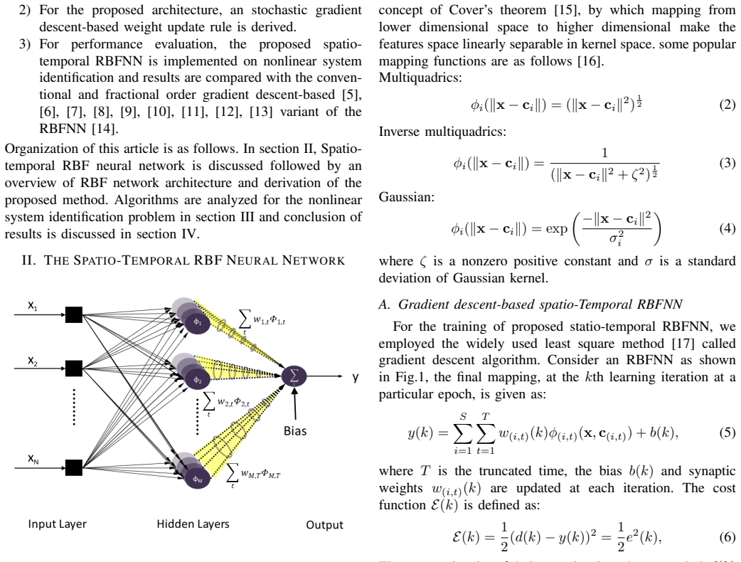
The central object is the spatio-temporal RBF hidden layer, whose output is $y(k)=\sum_{i=1}^S\sum_{t=1}^T w_{i,t}(k)\varphi_{i,t}(x,c_{i,t})+b(k)$. Each hidden unit carries both a spatial index $i$ and a temporal index $t$, giving $S\times T$ effective units, and the weight update derived from the squared-error cost is $w_{i,t}(k+1)=w_{i,t}(k)+\eta\,\varphi_{i,t}(x,c_{i,t})e(k)$. The mechanism carries the argument because every reported learning curve is a direct test of whether this re-indexed expansion plus the associated weight update identifies the nonlinear system.

What would settle it

Run the same nonlinear system identification task with the standard RBF given the same learning rate $10^{-2}$, the same $S\times T$ hidden units, and the same basis function used for $\varphi_{i,t}$, holding every other setting fixed. If the standard RBF then reaches approximately the same training and test MSE as the spatio-temporal RBF, the reported advantage is not due to the spatio-temporal architecture.

Watch

Extended reading notes

Core claim

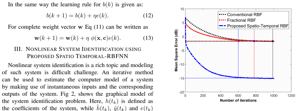
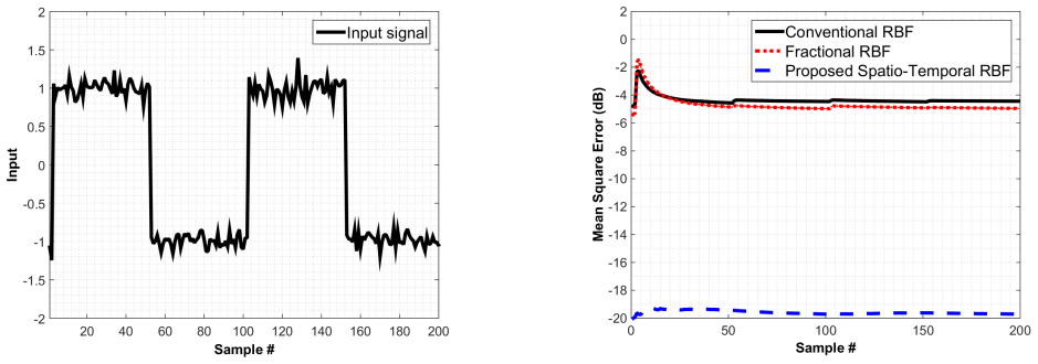
The paper's central claim is that separating time and space in the RBF hidden layer—modeling temporal dynamics with one index and spatial nonlinearity with another—yields a substantially better nonlinear system identifier than the standard architecture under gradient-descent training. The proposed model replaces $y=\sum_{i=1}^S w_i\varphi_i(\|x-c_i\|)+b$ by $y(k)=\sum_{i=1}^S\sum_{t=1}^T w_{i,t}(k)\varphi_{i,t}(x,c_{i,t})+b(k)$, and the weight update becomes $w_{i,t}(k+1)=w_{i,t}(k)+\eta\,\varphi_{i,t}(x,c_{i,t})e(k)$. The authors interpret this as exploiting time-space orthogonality, and they report that the spatio-temporal network reaches a training MSE of $-15.1286$ dB and a test MSE of $-19.67$ dB, against $-1.6813$ dB training and $-4.431$ dB test for the conventional RBF, and $-1.7444$ dB training and $-4.955$ dB test for the fractional RBF. The stated conclusion is that the spatio-temporal architecture, trained by the same gradient-descent rule adapted to the double sum, is what delivers the improvement.

Load-bearing premise

The comparison assumes that the reported gain comes from the spatio-temporal indexing, but the simulations also use a much larger learning rate ($10^{-2}$ versus $2\times10^{-5}$), more hidden units ($S\times T$ versus $S$), and leave $T$ and the exact $\varphi_{i,t}(x,c_{i,t})$ unspecified; if those changes, not the indexing, produce the gain, the central claim collapses.

Editorial extensions

If this is right

On temporal system-identification tasks, substituting the double-sum spatio-temporal hidden layer for the standard RBF layer should yield lower steady-state error and faster convergence under the same squared-error cost.
The derived update rule is online and local, so it can be dropped into existing RBF training loops with negligible extra computation.
Because the derivation uses only the chain rule, the same spatio-temporal indexing applies to any differentiable kernel, such as Gaussian, multiquadric, or inverse multiquadric, and to gradient variants including fractional-order updates.
The approach preserves RBF's light data requirement and simple three-layer structure, so it offers a low-cost alternative to deep architectures for nonlinear identification.

Reading between the lines

Editorial extensions of the paper, not claims the author makes directly.

The reported comparison changes several variables at once—learning rate ($10^{-2}$ versus $2\times10^{-5}$), number of hidden units ($S\times T$ versus $S$), and the unspecified $T$ and $\varphi_{i,t}$—so the size of the architectural contribution is an open question; a controlled ablation with matched learning rate and matched parameter count is the natural next experiment.
If the benefit is genuinely architectural, the temporal index likely acts as an embedded delay line, making the spatio-temporal RBF a kernelized relative of tapped-delay-line and temporal-convolution models; this connection is not explored in the paper.
A direct testable extension is to report $T$ and the explicit form of $\varphi_{i,t}(x,c_{i,t})$, since the paper leaves both undefined; specifying them would let others reproduce the network exactly.

Share X Bluesky LinkedIn Reddit HN

Signed reviews

No signed human review yet.

Editorial analysis

A structured set of objections, weighed in public.

Desk editor's note, referee report, and a circularity audit.

Desk Editor's Note

read the letter

Colleague,

The short version: this paper is a re-indexing of the RBF output from S hidden units to S×T hidden units, with T never defined and the basis function φ(i,t) never specified. The derivation of the weight update reduces to the standard RBF delta rule. The empirical section claims a ~15 dB test-MSE improvement over conventional and fractional RBF baselines, but that comparison is badly confounded.

What is actually new: essentially nothing architecturally. Equation (5) is Eq. (1) with the index range changed, and Eq. (11) is textbook gradient descent for an RBF. The authors do not explain how the temporal index enters the kernel, so the "spatio-temporal" label is doing no mathematical work. The paper is at least clearly written, and the derivation, such as it is, is algebraically correct. They also posted MATLAB code, which is more than many submissions do.

The soft spots are the load-bearing ones. The proposed ST-RBF runs with learning rate η=1e-2 while the baselines use η=2e-5 — a 500× difference that alone could explain the entire gap. The text even says the proposed η is "half" of the baseline, which is internally inconsistent. The proposed network has S×T hidden units versus S=6 for the baselines, adding capacity. T is never defined. No error bars or variance are reported despite 1000 Monte Carlo runs, so the −19.67 dB figure is just one number. The stress-test note is right: matching the learning rate and using an ordinary RBF with S×T hidden units would likely reproduce the reported gains, making the claimed architectural benefit an artifact of hyperparameter choice.

I don't see circularity in the derivation, and the test signal is separate from training, so the problem is confounding, not fitting-to-the-test-set. The citation pattern is heavy self-citation, but that is common and not disqualifying by itself.

My take: this is not ready for publication. The empirical claim is unsupported as stated, and the novel content is a renamed increase in hidden units. A revision with a defined architecture, matched hyperparameters, equal capacity, and error bars could be reconsidered, but that is a re-do of the experiments, not a patch. I would not send it to peer review in its current form. For you: if you care about RBF variants for nonlinear system identification, the paper is a cautionary example of how not to run comparisons. No need to cite it.

Best, [You]

Referee Report

4 major / 4 minor

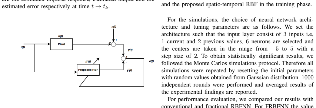
Summary. The manuscript proposes a 'spatio-temporal RBF neural network' for nonlinear system identification. The network extends the standard RBF output sum in Eq. (1) to a double sum over spatial index i and temporal index t in Eq. (5), and the authors derive a gradient-descent update rule in Eqs. (8)-(13). The paper evaluates the method on a single simulated nonlinear system described by Eq. (14), comparing against a conventional RBF and a fractional-gradient RBF. Reported training MSEs are -15.1286 dB for the proposed method versus -1.6813 dB (RBF) and -1.7444 dB (FRBF); test MSEs are -19.67 dB versus -4.431 dB and -4.955 dB, respectively, averaged over 1000 Monte Carlo rounds.

Significance. If the reported gains were real, a simple re-indexing of RBF hidden units to incorporate temporal structure would be a practically useful contribution for nonlinear system identification. The paper also provides a link to the implementation, which is a positive reproducibility feature, and it fixes the nonlinear system and input signal explicitly. However, the current evidence does not support the central claim. The learning-rate update in Eq. (11) is the standard delta rule with a re-indexed weight, so the theoretical contribution is not new. The empirical comparison is confounded by a 500x difference in learning rate, an undefined temporal expansion with an increased number of hidden units, and a lack of error bars. The significance of the architecture itself is therefore not established in this manuscript.

major comments (4)

[Section III, simulation setup] The reported performance advantage is confounded with a 500x larger learning rate. The proposed ST-RBF uses eta = 1e-2, while both baselines use eta = eta_v = 2e-5. A larger step size alone can plausibly move a gradient-descent method from a poorly converged steady-state MSE near -1.7 dB to a much lower error, independent of any architectural benefit. The comparison must include baselines trained with the same learning rate (or a learning-rate sweep) and the same number of effective hidden units to isolate the effect of the spatio-temporal indexing. As written, the claim in the abstract that ST-RBF achieves 'significantly reduced estimation error' is not supported.
[Section II, Eq. (5)] The proposed model is not fully specified. The basis functions phi_(i,t)(x, c_(i,t)) and the centers c_(i,t) are never defined; the only basis functions given in Eqs. (2)-(4) are functions of x and c_i without the temporal index. The truncation parameter T is also never assigned a numerical value or explained. Without these definitions, the architecture in Eq. (5) cannot be reproduced or tested, and the question of whether the double index (i,t) represents a true temporal expansion or merely a larger static basis cannot be answered. Additionally, Eq. (5) sums over S*T terms, so the comparison against a baseline with S=6 hidden units changes network capacity as well as architecture.
[Section III, test-phase MSE reporting] The paper claims 1000 independent Monte Carlo rounds, but reports only the mean training and test MSE values with no variance, confidence intervals, or statistical significance tests. Without this information, the difference between -19.67 dB and -4.431 dB cannot be distinguished from a hyperparameter artifact. The statement that the proposed method 'outperforms' the baselines is therefore not statistically substantiated.
[Section III, learning-rate sentence] The text says the proposed ST-RBF learning rate is 'half of the RBF and FRBF learning rates i.e., 1e-2', but the baseline learning rate is 2e-5, so 'half' would be 1e-5, not 1e-2. This internal inconsistency suggests the 500x increase may be unintentional, and it further undermines confidence in the experimental setup. The authors should correct the statement or the value and explain which setting was actually used.

minor comments (4)

[Section II.A, heading] The heading contains the typo 'statio-temporal RBFNN' and should read 'spatio-temporal RBFNN'.
[Section III, testing paragraph] The phrase 'calclulated' should be 'calculated'.
[Section III, simulation setup] The phrase 'Monte Carlos simulations protocol' is nonstandard; it should be 'Monte Carlo simulation protocol'.
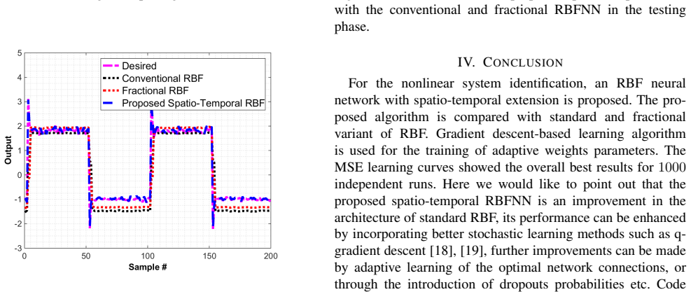
[Section III, Fig. 5] The claim that the proposed output 'shows the exact match' is qualitative; a quantitative error metric or a zoomed plot would be more informative.

Circularity Check

0 steps flagged · score 0.0 of 10

No circular derivation: the weight update and test MSE are independent of the claimed improvement, so the paper's central issue is an experimental confound, not circularity.

full rationale

The derivation chain is self-contained. Section II defines the proposed network as a double sum over S spatial and T temporal indices (Eq. 5) and applies the usual chain rule to obtain the delta rule w(i,t)(k+1)=w(i,t)(k)+ηφ(i,t)(x,c(i,t))e(k) (Eq. 11). This is not a restatement of the training target or of the performance claim; it is the standard gradient-descent update for the re-indexed architecture. The reported training and test MSE values (Section III) are computed by simulation on the system in Eq. (14), with the test phase using a separate 200-sample signal, so the −19.67 dB test figure is not the minimized training cost by construction. The fractional-RBF baselines are implemented in the paper rather than imported as a theorem, and the self-citations [5]–[14] are literature pointers to fractional-gradient variants, not load-bearing assumptions that force the ST-RBF result. The serious weakness in the empirical comparison is confounding: the proposed run uses η=1×10−2 versus 2×10−5 for the baselines and S×T hidden units versus S=6, while T and φ(i,t) are left unspecified (Eq. (5) and Section III). The text also says 1×10−2 is half of 2×10−5, which is arithmetically inconsistent. These are correctness and experimental-design problems, not circularity: no equation in the paper reduces the claimed advantage to the input data or to a fitted parameter renamed as a prediction.

Assumptions & free parameters 6 free parameters · 4 assumptions · 0 invented entities

The ledger is mostly standard: the arithmetic in the weight update is elementary, so no exotic axioms are needed. The fragility is experimental and architectural: T and phi_i,t are undefined, the hyperparameters are hand-picked, and the baseline comparison does not control for learning rate or model size.

free parameters (6)

Proposed ST-RBF learning rate eta = 1e-2
Assigned by the authors; no grid search or sensitivity analysis is reported, and it differs by a factor of 500 from the baselines.
Baseline learning rates eta and eta_v = 2e-5
Used for RBF and FRBF; the mismatch with the proposed rate makes the comparison unfair.
RBF center set = -5 to 5 in steps of 2 (six centers)
Chosen by hand; changes model capacity and can determine part of the performance gap.
Gaussian spread sigma = 1
Chosen without sensitivity analysis; kernel width affects fit quality.
Temporal truncation T = Not stated
Eq. (5) sums over T but the paper never gives its value; if the shipped code sets it, it is still a tuned model-size parameter.
Fractional baseline parameters alpha and nu = alpha=0.5, nu=0.9
These configure the FRBF baseline only; they are arbitrary but not central to the proposed method.

assumptions (4)

standard math The gradient of the cost is computed with the standard chain rule and the RBF output is linear in the weights.
Eqs. (9)-(11) rely only on elementary calculus; this part is correct.
domain assumption The chosen benchmark (Eq. 14) and the step-like training/test signals are representative of general nonlinear system identification.
Only one system and one input design are tested; no justification is given that results extend to other systems.
ad hoc to paper The double index (i,t) can separate temporal dynamics from spatial nonlinearity without further structure.
The paper invokes 'time-space orthogonality' but Eq. (5) is just a double sum over weights; no separability condition or mathematical statement of orthogonality is given.
ad hoc to paper The basis functions phi_i,t(x,c_i,t) are well-defined and valid kernels.
No definition for phi_i,t is provided; readers cannot tell whether time enters the argument, the center, or the kernel shape.

how reviews work

0 comments

Cite this review

Pith. "Pith review of Spatio-Temporal RBF Neural Networks." pith.science (2026). https://pith.science/paper/JNFGISTW

@misc{pith2026190801321,
  author       = {Pith},
  title        = {Pith review of: Spatio-Temporal RBF Neural Networks},
  year         = {2026},
  howpublished = {\url{https://pith.science/paper/JNFGISTW}},
  note         = {Machine review of arXiv:1908.01321}
}

read the original abstract

Herein, we propose a spatio-temporal extension of RBFNN for nonlinear system identification problem. The proposed algorithm employs the concept of time-space orthogonality and separately models the dynamics and nonlinear complexities of the system. The proposed RBF architecture is explored for the estimation of a highly nonlinear system and results are compared with the standard architecture for both the conventional and fractional gradient decent-based learning rules. The spatio-temporal RBF is shown to perform better than the standard and fractional RBFNNs by achieving fast convergence and significantly reduced estimation error.

Figures

Figures reproduced from arXiv: 1908.01321 by the authors.

**Figure 3.** MSE behavior of the conventional RBF, Fractional RBF [PITH_FULL_IMAGE:figures/full_fig_p003_3.png] view at source ↗

**Figure 2.** Modelling of non-linear system using adaptive learning [PITH_FULL_IMAGE:figures/full_fig_p003_2.png] view at source ↗

Figures from the paper (2 more)

**Figure 6.** Figure 6: MSE behaviour of the proposed spatio-temporal RBF [PITH_FULL_IMAGE:figures/full_fig_p004_6.png]

**Figure 5.** Figure 5: Comparison of model and actual output. Finally the MSE in test phase is calclulated for 1000 independent rounds and mean value of MSE is reported for different noisy test inputs. In [PITH_FULL_IMAGE:figures/full_fig_p004_5.png]

Discussion (0). Continue with ORCID to comment.

Reference graph

Works this paper leans on

20 extracted references · 4 canonical work pages

[1]

Rafp-pred: Robust prediction of antifreeze proteins using localized analysis of n-peptide compositions,

S. Khan, I. Naseem, R. Togneri, and M. Bennamoun, “Rafp-pred: Robust prediction of antifreeze proteins using localized analysis of n-peptide compositions,” IEEE/ACM Transactions on Computational Biology and Bioinformatics, vol. PP, no. 99, pp. 1–1, 2017

2017
[2]

Ecmsrc: A sparse learning approach for the prediction of extracellular matrix proteins,

I. Naseem, S. Khan, R. Togneri, and M. Bennamoun, “Ecmsrc: A sparse learning approach for the prediction of extracellular matrix proteins,” Current Bioinformatics, vol. 12, no. 4, pp. 361–368, 2017

2017
[3]

Efﬁcient b-mode ultrasound image reconstruction from sub-sampled rf data using deep learning,

Y . H. Yoon, S. Khan, J. Huh, J. C. Yeet al., “Efﬁcient b-mode ultrasound image reconstruction from sub-sampled rf data using deep learning,” IEEE transactions on medical imaging , 2018

2018
[4]

A novel adaptive kernel for the rbf neural networks,

S. Khan, I. Naseem, R. Togneri, and M. Bennamoun, “A novel adaptive kernel for the rbf neural networks,” Circuits, Systems, and Signal Processing, pp. 1–15, 2016

2016
[5]

A novel fractional gradient-based learning algorithm for recurrent neural networks,

S. Khan, J. Ahmad, I. Naseem, and M. Moinuddin, “A novel fractional gradient-based learning algorithm for recurrent neural networks,” Cir- cuits, Systems, and Signal Processing , pp. 1–20, 2017

2017
[6]

VP- FLMS: a novel variable power fractional LMS algorithm,

S. Khan, M. Usman, I. Naseem, R. Togneri, and M. Bennamoun, “VP- FLMS: a novel variable power fractional LMS algorithm,” in 2017 Ninth International Conference on Ubiquitous and Future Networks (ICUFN) (ICUFN 2017) , Milan, Italy, Jul. 2017

work page 2017
[7]

A robust variable step size fractional least mean square (rvss- ﬂms) algorithm,

——, “A robust variable step size fractional least mean square (rvss- ﬂms) algorithm,” in 13th IEEE Colloquium on Signal Processing and its Applications (CSPA 2017) . IEEE, 2017

2017
[8]

Rvp- ﬂms : A robust variable power fractional lms algorithm,

J. Ahmad, M. Usman, S. Khan, I. Naseem, and H. J. Syed, “Rvp- ﬂms : A robust variable power fractional lms algorithm,” in 2016 IEEE International Conference on Control System, Computing and Engineering (ICCSCE) . IEEE, 2016

work page 2016

Show all 20 references

[9]

Fclms: Fractional complex lms algorithm for complex system identiﬁcation,

J. Ahmad, S. Khan, M. Usman, I. Naseem, M. Moinuddin, and H. J. Syed, “Fclms: Fractional complex lms algorithm for complex system identiﬁcation,” in Signal Processing & its Applications (CSPA), 2017 IEEE 13th International Colloquium on . IEEE, 2017, pp. 39–43

2017
[10]

Flmf: Fractional least mean fourth algorithm for channel esti- mation in non-gaussian environment,

S. Khan, N. Ahmed, M. A. Malik, I. Naseem, R. Togneri, and M. Ben- namoun, “Flmf: Fractional least mean fourth algorithm for channel esti- mation in non-gaussian environment,” in 2017 International Conference on Information and Communication Technology Convergence (ICTC) , Oct...

2017
[11]

Comments on

S. Khan, A. Wahab, I. Naseem, and M. Moinuddin, “Comments on” design of fractional-order variants of complex lms and nlms algorithms for adaptive channel equalization”,” arXiv preprint arXiv:1802.09252 , 2018

2018 arXiv
[12]

Comments on

S. Khan, I. Naseem, A. Sadiq, J. Ahmad, and M. Moinuddin, “Comments on” momentum fractional lms for power signal parameter estimation”,” arXiv preprint arXiv:1805.07640 , 2018

2018 arXiv
[13]

Comments and corrections comments on“fractional extreme value adaptive training method: Fractional steepest descent approach

A. Wahab and S. Khan, “Comments and corrections comments on“fractional extreme value adaptive training method: Fractional steepest descent approach”,” IEEE transactions on neural networks and learning systems, 2019

2019
[14]

A fractional gradient descent-based rbf neural network,

S. Khan, I. Naseem, M. A. Malik, R. Togneri, and M. Bennamoun, “A fractional gradient descent-based rbf neural network,” Circuits, Systems, and Signal Processing , pp. 1–22, 2018

2018
[15]

Geometrical and statistical properties of systems of linear inequalities with applications in pattern recognition,

T. M. Cover, “Geometrical and statistical properties of systems of linear inequalities with applications in pattern recognition,” IEEE Transactions on Electronic Computers , vol. EC-14, no. 3, pp. 326–334, June 1965

1965
[16]

Haykin, Neural Networks: A Comprehensive F oundation , 2nd ed

S. Haykin, Neural Networks: A Comprehensive F oundation , 2nd ed. Upper Saddle River, NJ, USA: Prentice Hall PTR, 1998

1998
[17]

Topological sensitivity based far-ﬁeld detection of elastic inclusions,

T. Abbas, S. Khan, M. Sajid, A. Wahab, and J. C. Ye, “Topological sensitivity based far-ﬁeld detection of elastic inclusions,” Results in physics, vol. 8, pp. 442–460, 2018

2018
[18]

En- hanced q-least mean square,

A. Sadiq, S. Khan, I. Naseem, R. Togneri, and M. Bennamoun, “En- hanced q-least mean square,” Circuits, Systems, and Signal Processing , pp. 1–23, 2019

2019
[19]

q-lmf: Quantum calculus-based least mean fourth algorithm,

A. Sadiq, M. Usman, S. Khan, I. Naseem, and M. Moinuddin, “q-lmf: Quantum calculus-based least mean fourth algorithm,” arXiv preprint arXiv:1812.02588, 2018

2018 arXiv
[20]

S. Khan. Nonlinear system identiﬁcation using spatio- temporal rbf-nn. Retrieved November 26, 2018. [Online]. Available: https://www.mathworks.com/matlabcentral/ﬁleexchange/ 68415-nonlinear-system-identiﬁcation-using-spatio-temporal-rbf-nn

2018

Pith tools

Reviewed August 14, 2026 · model on record in the stance chip above.

[1] [1]

Rafp-pred: Robust prediction of antifreeze proteins using localized analysis of n-peptide compositions,

S. Khan, I. Naseem, R. Togneri, and M. Bennamoun, “Rafp-pred: Robust prediction of antifreeze proteins using localized analysis of n-peptide compositions,” IEEE/ACM Transactions on Computational Biology and Bioinformatics, vol. PP, no. 99, pp. 1–1, 2017

2017

[2] [2]

Ecmsrc: A sparse learning approach for the prediction of extracellular matrix proteins,

I. Naseem, S. Khan, R. Togneri, and M. Bennamoun, “Ecmsrc: A sparse learning approach for the prediction of extracellular matrix proteins,” Current Bioinformatics, vol. 12, no. 4, pp. 361–368, 2017

2017

[3] [3]

Efﬁcient b-mode ultrasound image reconstruction from sub-sampled rf data using deep learning,

Y . H. Yoon, S. Khan, J. Huh, J. C. Yeet al., “Efﬁcient b-mode ultrasound image reconstruction from sub-sampled rf data using deep learning,” IEEE transactions on medical imaging , 2018

2018

[4] [4]

A novel adaptive kernel for the rbf neural networks,

S. Khan, I. Naseem, R. Togneri, and M. Bennamoun, “A novel adaptive kernel for the rbf neural networks,” Circuits, Systems, and Signal Processing, pp. 1–15, 2016

2016

[5] [5]

A novel fractional gradient-based learning algorithm for recurrent neural networks,

S. Khan, J. Ahmad, I. Naseem, and M. Moinuddin, “A novel fractional gradient-based learning algorithm for recurrent neural networks,” Cir- cuits, Systems, and Signal Processing , pp. 1–20, 2017

2017

[6] [6]

VP- FLMS: a novel variable power fractional LMS algorithm,

S. Khan, M. Usman, I. Naseem, R. Togneri, and M. Bennamoun, “VP- FLMS: a novel variable power fractional LMS algorithm,” in 2017 Ninth International Conference on Ubiquitous and Future Networks (ICUFN) (ICUFN 2017) , Milan, Italy, Jul. 2017

work page 2017

[7] [7]

A robust variable step size fractional least mean square (rvss- ﬂms) algorithm,

——, “A robust variable step size fractional least mean square (rvss- ﬂms) algorithm,” in 13th IEEE Colloquium on Signal Processing and its Applications (CSPA 2017) . IEEE, 2017

2017

[8] [8]

Rvp- ﬂms : A robust variable power fractional lms algorithm,

J. Ahmad, M. Usman, S. Khan, I. Naseem, and H. J. Syed, “Rvp- ﬂms : A robust variable power fractional lms algorithm,” in 2016 IEEE International Conference on Control System, Computing and Engineering (ICCSCE) . IEEE, 2016

work page 2016