REVIEW 4 major objections 5 minor 74 references
Twisted bilayer graphene: low-energy physics, electronic and optical properties
T0 review · 4 major / 5 minor · reviewed 2026-08-14 · deepseek-v4-flash
Pith's one-line read The paper establishes that a continuum model retaining only three interlayer momentum-transfer processes reproduces the low-energy band structure, Fermi velocity renormalization, optical conductivity, and surface plasmon-polariton…
desk verdict Useful pedagogical review of the continuum model for twisted bilayer graphene, but the central Fermi-velocity formula has an internal factor-of-9 inconsistency that must be fixed before the chapter can be trusted as a reference. read the letter →
The pith
A machine-rendered reading of the paper's core claim, the machinery that carries it, and where it could break.
The reading
What carries the argument
The central object is the moiré-reciprocal-space Hamiltonian: an expansion of the two layers' Dirac states in Bloch waves shifted by moiré reciprocal lattice vectors, coupled by the three interlayer momentum transfers $\mathbf{q}_b$, $\mathbf{q}_{tr}$, and $\mathbf{q}_{tl}$, whose amplitudes come from the rapidly decaying Fourier transform $t_\perp(\mathbf{p})$ of the Slater-Koster interlayer hopping. Truncating the lattice of moiré reciprocal vectors to ten sites turns the problem into a $20\times20$ matrix eigenvalue problem whose bands give the density of states, carrier density, Drude weight, and optical conductivity; the surface plasmon-polariton dispersion then follows by inserting that conductivity into the transverse-magnetic boundary-condition equation.
What would settle it
Evaluate $t_\perp(\mathbf{p})$ from first principles at the momenta of the next-order umklapp processes, $|\mathbf{p}| \approx |\mathbf{K}|$ plus a moiré reciprocal vector, and compare with $t_\perp(|\mathbf{K}|)$; if any of those amplitudes exceeds even a few percent of $t_\perp(|\mathbf{K}|)$, the truncated three-process model's bands and conductivity would shift measurably.
Extended reading notes
Core claim
On its own terms, this chapter claims that twisted bilayer graphene's low-energy physics is a three-process story: after expanding in Bloch states built from each layer's Dirac points, the interlayer coupling reduces to the three momentum transfers $\mathbf{q}_b$, $\mathbf{q}_{tr}$, and $\mathbf{q}_{tl}$, whose amplitudes are all set by $t_\perp(|\mathbf{K}|)/A_{u.c.}$ times phase factors. The moiré band structure is the spectrum of a matrix Hamiltonian over moiré reciprocal lattice vectors, and the paper shows this reproduces the perturbative Fermi velocity renormalization $v_F^*/v_F = 1 - \left(\frac{t_\perp(|\mathbf{K}|)}{v_F\hbar|\mathbf{K}|A_{u.c.}}\right)^2\frac{1}{4\sin^2(\theta/2)}$, brings van Hove singularities down to low energy, and yields an optical conductivity whose Drude weight is computed from band velocities and whose imaginary regular part is fixed by a regularized Kramers-Kronig relation. The same conductivity then produces the surface plasmon-polariton dispersion through the standard transverse-magnetic boundary-condition equation, recovering known graphene results and giving a qualitatively different dispersion at $\theta = 1.8^\circ$.
Load-bearing premise
The calculation stands on the assumption that only three interlayer momentum-transfer processes matter because the interlayer hopping $t_\perp(\mathbf{p})$ decays very quickly with momentum; if the decay is slower than assumed, or the Slater-Koster decay constants $q_\pi$ and $q_\sigma$ are not related in the way the paper sets them, the band structure, conductivity, and plasmon dispersion would all change.
Editorial extensions
If this is right
- Twist angle becomes a continuous tuning knob: van Hove singularities move to experimentally accessible energies, which is what makes doping-driven instabilities plausible in these systems.
- The Fermi velocity renormalization of Eq. (103) predicts a measurable angle-dependent reduction of the low-energy slope, with a formal vanishing at magic angles that signals the breakdown of the perturbative description.
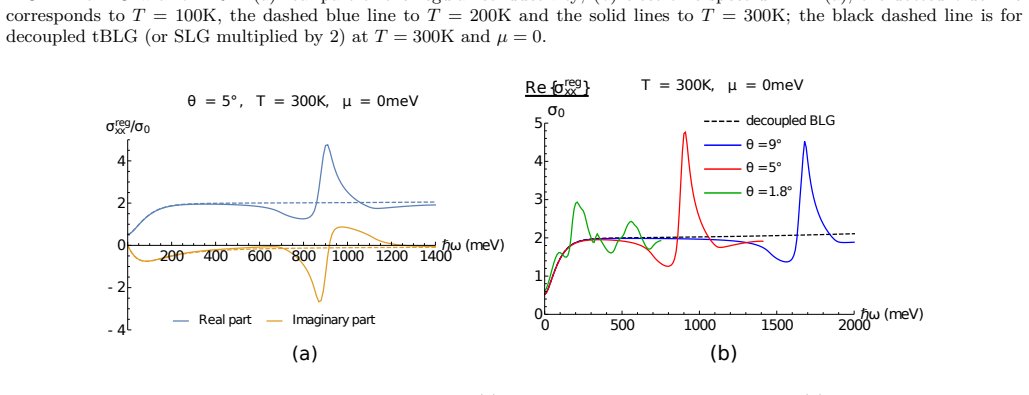
- The optical conductivity acquires an angle-dependent low-energy peak from the active van Hove transitions, while other symmetry-related transitions remain dark, as earlier calculations found.
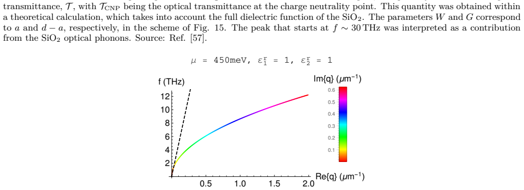
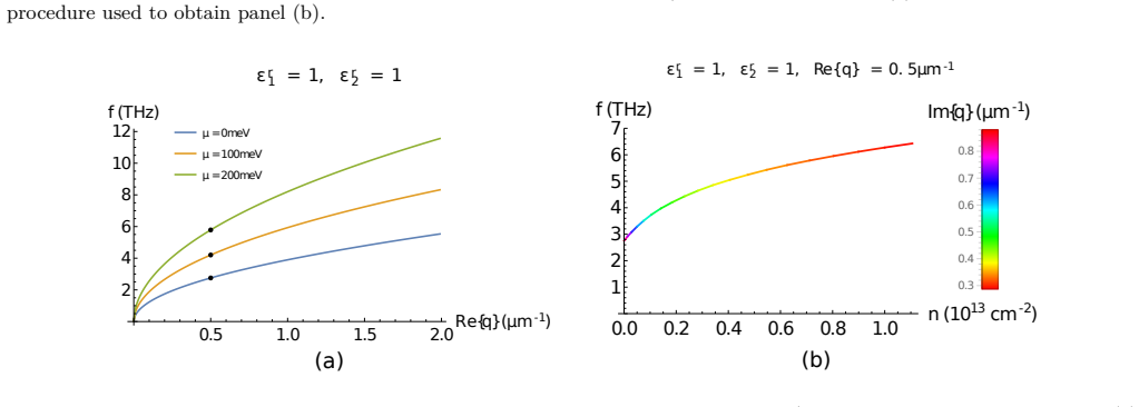
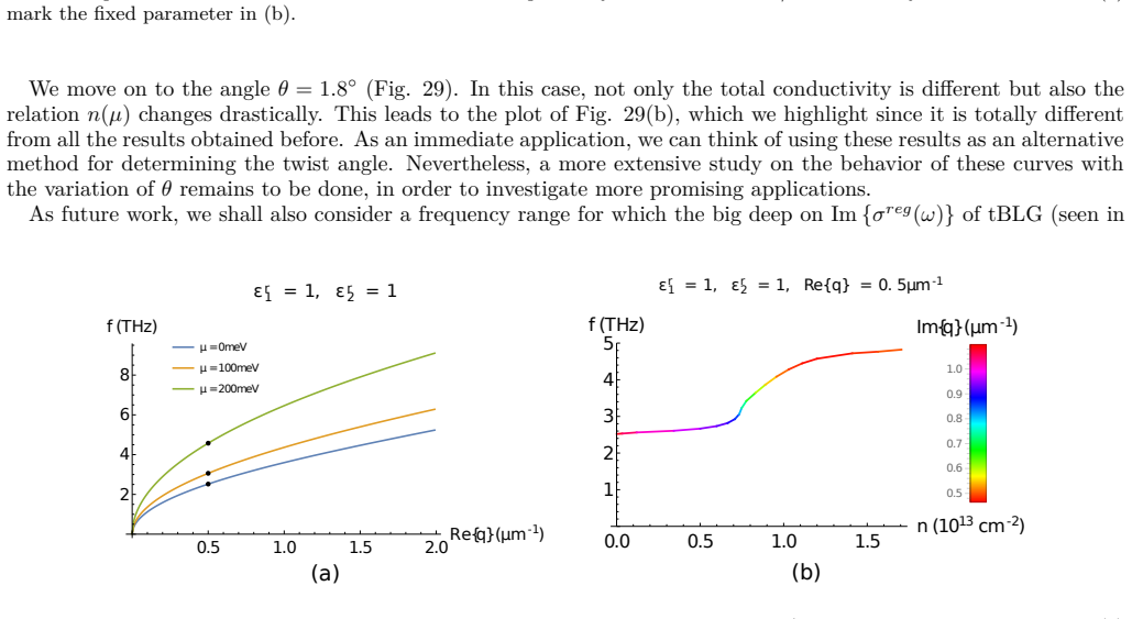
- For larger angles such as $\theta \approx 9^\circ$, the surface plasmon-polariton response of tBLG resembles that of decoupled bilayer graphene, but at $\theta \approx 1.8^\circ$ the frequency-versus-density dispersion changes qualitatively, allowing twist-angle determination from plasmonic measurements.
- In frequency windows where the imaginary part of the total conductivity becomes negative, transverse-magnetic surface plasmons cannot exist; the paper points to transverse-electric modes and a possible polarizer application.
Reading between the lines
- The same three-process truncation should transfer to other twisted or lattice-mismatched van der Waals bilayers, such as graphene on hexagonal boron nitride, whenever the interlayer hopping in momentum space is equally sharply peaked; the observable signature would be the same kind of angle-tunable van Hove and plasmon features.
- The paper's angle-dependent SPP dispersion at $\theta = 1.8^\circ$ suggests a contact-free metrology: extracting the twist angle from a measured plasmon frequency-versus-density curve could complement STM and diffraction, though the paper only offers this as an immediate application, not a demonstrated method.
- Because the regularized Kramers-Kronig prescription fixes the imaginary conductivity for any truncated effective model, it is likely to become a standard tool beyond tBLG, for example in other moiré systems where the full tight-binding model is too large.
- Near magic-angle twists the perturbative Fermi-velocity formula breaks down exactly where flat bands appear; this points to a non-perturbative calculation of the conductivity and SPP response at $\theta \lesssim 1.05^\circ$ as the natural next step, likely showing interaction-enhanced features absent from the present single-particle treatment.
Signed reviews
Editorial analysis
A structured set of objections, weighed in public.
Referee Report
Summary. This manuscript is a pedagogical chapter on the low-energy continuum theory of twisted bilayer graphene (tBLG). It derives the moiré geometry, builds an interlayer Hamiltonian via generalized umklapp processes, truncates the coupling to three dominant momentum transfers, and from this obtains a renormalized Fermi velocity, the low-energy band structure with van Hove singularities, the optical conductivity (Drude and regular parts), and the surface plasmon-polariton dispersion. The chapter also benchmarks parts of the calculation against single-layer and Bernal bilayer graphene results, against the experimental DC conductivity of Cao et al., and against earlier continuum and tight-binding studies.
Significance. If the derived formulas and numerical protocols were correct, the chapter would be a useful self-contained pedagogical reference: it gives a detailed derivation of the interlayer Hamiltonian, a clear treatment of the folded-zone structure, a general tight-binding-based linear-response framework for the optical conductivity, and a comparison of plasmon dispersions for different twist angles. The strengths of the manuscript are its explicit derivations, its cross-checks against known SLG and Bernal bilayer limits, and its comparison with published experimental and numerical results. However, the central analytic result for the Fermi-velocity renormalization contains an algebraic inconsistency that must be resolved before the pedagogical claims can be accepted.
major comments (4)
- [III C 1, Eqs. (102)-(103)] The two printed expressions for the renormalized Fermi velocity are mutually inconsistent. With α defined as in Eq. (102), Eq. (102) gives v*_F/v_F = 1 − 9α², whereas Eq. (103) is algebraically equal to 1 − α² because |ΔK| = 2|K| sin(θ/2). Moreover, neither value is compatible with the text's statement that flat bands appear at θ ≲ 1.05°: using t⊥(|K|) = 0.58 eV Ų, A_u.c. = 5.24 Ų, and ℏv_F|K| ≈ 10.8 eV, Eq. (103) vanishes near θ ≈ 0.59°, Eq. (102) near θ ≈ 1.77°, while the standard 1 − 3α² condition vanishes near θ ≈ 1.05°. The derivation must be corrected and the advertised match to the known result of Ref. [11] re-established; this is a load-bearing point for the pedagogical claim of Section III.
- [III B 4, Eqs. (79)-(89)] The reduction of the generalized umklapp sum in Eq. (70) to the three momenta q_b, q_tr, q_tl is justified only by the qualitative statement that t⊥(p) decays rapidly (Fig. 10). Since this truncation is the basis for the Hamiltonian of Eq. (107) and hence for all band-structure, conductivity, and plasmon results, the manuscript should quantify the truncation error, for example by including additional moiré reciprocal-lattice shells and showing convergence of the low-energy bands and of the optical conductivity for representative angles θ = 9°, 5°, and 1.8°.
- [III B 3, Eq. (76)] The Slater-Koster decay parameter qσ is fixed by assuming equal spatial decay coefficients qπ/d = qσ/d⊥, an assumption with no independent microscopic justification. Because t⊥(p) and hence the effective interlayer coupling depend on qσ, the quantitative predictions (magic-angle position, Drude weight dips, SPP frequencies) inherit this uncertainty. A sensitivity analysis over the plausible range of qσ, or an independent determination of qσ, would materially strengthen the model.
- [IV A 1, Eq. (150)] The regularized Kramers-Kronig formula subtracts the high-frequency constant 2σ0 and then imposes a finite cut-off Λ, but no argument is given that this subtraction is unique for the truncated low-energy model or that the final results are insensitive to Λ and to the precise treatment of the tail. Since the imaginary part of the conductivity enters Eq. (165) for the SPP dispersion (Figs. 28-29), the sensitivity of the SPP curves to the regularization procedure should be documented.
minor comments (5)
- [Page 2, Introduction] The phrase 'ab initionumerical' should read 'ab initio numerical'.
- [Page 22, IV A 1] 'Sublattice indeces' should be 'sublattice indices'.
- [Fig. 10] The horizontal axis label 'p(Å-1)' should read '|p| (Å⁻¹)' because t⊥(p) is defined as a function of |p|.
- [Fig. 15 caption] The word 'satisfty' should be 'satisfy'.
- [Eq. (112) versus Eq. (114)] The sign convention in the Peierls phase should be checked for consistency with the substitution k + (e/ℏ)A in Eq. (114); a brief note explaining the sign choice would help readers.
Circularity Check
No circularity: the paper re-derives the continuum model, benchmarks against prior external results, and the factor-9 discrepancy flagged by the skeptic is a correctness issue, not a circular one.
full rationale
The derivation is self-contained rather than circular. The chapter constructs the interlayer Hamiltonian from a tight-binding starting point, derives the three dominant umklapp couplings, and then computes the Fermi-velocity renormalization, band structure, density of states, optical conductivity, and plasmon dispersion without fitting those outputs to the model inputs. The value t⊥(|K|) is fixed by the independent Bernal-stacking limit t⊥ = 0.33 eV through Eq. (92), and the same constant is then used in the velocity formula and in the numerical calculations, so the predicted quantities are not redefinitions of the fitted parameter. Self-citations appear (Refs. [11], [12], [47]), but they are not load-bearing: the model is re-derived in Sections III B and III C, the velocity result is derived perturbatively in Eq. (100)-(103), and the plasmon derivation follows the standard textbook treatment of Ref. [47] explicitly rather than assuming its conclusion. The magic-angle statement is cited to Bistritzer and MacDonald, but no computation in the chapter relies on that citation as a premise. The truncation to three umklapp processes is an approximation whose validity is discussed, not a parameter tuned to reproduce the claimed results. The skeptic's noted factor-of-9 inconsistency between Eqs. (102) and (103) is an internal algebraic or typographical error in the printed coefficient, not a case where a prediction reduces to an input by construction; it would be a correctness concern, not a circularity concern.
Assumptions & free parameters
free parameters (3)
- qπ =
3.15
- qσ =
7.42
- Γ =
16 meV
assumptions (7)
- domain assumption Single-orbital nearest-neighbor tight-binding model for graphene
- domain assumption Two-center approximation for interlayer hopping
- domain assumption Dirac cone approximation for low-energy states
- domain assumption Only three umklapp processes contribute to interlayer coupling
- ad hoc to paper Equal spatial decay coefficients qπ/d = qσ/d⊥
- domain assumption Incommensurate structure properties are independent of in-plane translation τ0
- domain assumption Regularization of the Kramers-Kronig relation using Re{σreg}→2σ0 at large frequency
Cite this review
Pith. "Pith review of Twisted bilayer graphene: low-energy physics, electronic and optical properties." pith.science (2026). https://pith.science/paper/4S4D2KDT
@misc{pith2026190801556,
  author       = {Pith},
  title        = {Pith review of: Twisted bilayer graphene: low-energy physics, electronic and optical properties},
  year         = {2026},
  howpublished = {\url{https://pith.science/paper/4S4D2KDT}},
  note         = {Machine review of arXiv:1908.01556}
}
read the original abstract
Van der Waals (vdW) heterostructures ---formed by stacking or growing two-dimensional (2D) crystals on top of each other--- have emerged as a new promising route to tailor and engineer the properties of 2D materials. Twisted bilayer graphene (tBLG), a simple vdW structure where the interference between two misaligned graphene lattices leads to the formation of a moir\'e pattern, is a test bed to study the effects of the interaction and misalignment between layers, key players for determining the electronic properties of these stackings. In this chapter, we present in a pedagogical way the general theory used to describe lattice mismatched and misaligned vdW structures. We apply it to the study of tBLG in the limit of small rotations and see how the coupling between the two layers leads both to an angle dependent renormalization of graphene's Fermi velocity and appearance of low-energy van Hove singularities. The optical response of this system is then addressed by computing the optical conductivity and the dispersion relation of tBLG surface plasmon-polaritons.
Figures

Figures from the paper (26 more)








Reference graph
Works this paper leans on
-
[11]
Results for twisted bilayer graphene A summary of the Drude weight results for tBLG is provided in Fig. 19. We stress that only the 2nd method was verified to work well for these computations. This happens because we are working with an effective Hamiltonian, as discussed before. Similarly to what we have seen for the SLG, we observe symmetric results for e...
work page 2000
-
[1]
Hamiltonian for rotated graphene monolayers We want to express the full Hamiltonian in terms of Bloch waves for the individual layers of the form of Eqs. (13) and (37), |ψ𝓁,k,α⟩= 1√N𝓁 R𝓁 eik·(R𝓁+τ𝓁,α)|𝓁,R𝓁,α⟩, (55) where 𝓁= 1, 2 labels the layer,α= A,B is the sublattice,N𝓁is the number of unit cells of each layer,R𝓁are the lattice sites,τ𝓁,αare the posi...
-
[2]
Tight-binding model To model this system, we retain the approximations used before for each individual layer; in addition, we take into account interlayer hopping, in a transversal tight-binding approximation between nearest-neighbors. We start by writing the Hamiltonian for the bilayer as a sum of three terms, H =H1 +H2 +H⊥, (32) where H𝓁is the Hamiltoni...
-
[3]
General interlayer Hamiltonian in terms of Bloch waves We write the interlayer Hamiltonian in second quantization in the basis of atomic-like localized states of each layer as V12 = R1,α,R2,β c† 1,α(R1)tαβ 12 (R1,R2)c2,β(R2), (59) where tαβ 12 (R1,R2) =⟨1,R1,α|H⊥|2,R2,β⟩ (60) is the interlayer hopping in the tight-binding basis. Writing the operators in...
-
[4]
Interlayer hopping for pz orbitals To make further progress, we must specify the functional form oftαβ 12 (r). First, since in graphene bothA and B sites correspond to the samepz orbital of carbon, we assumetAA 12 (r) =tBB 12 (r) =tAB 12 (r) =tBA 12 (r) =t⊥(r). In the two-center approximation, we expresst⊥(r) in terms of Slater-Koster parameters [30],Vppσ...
-
[5]
Interlayer Hamiltonian for small twist angles We now wish to specialize to the case of tBLG in the limit of small twist angles. For smallθ, the Dirac points K1 and K2 are close to each other and we can neglect coupling between K𝓁and−K𝓁points. If we are only interested in low-energy physics we can expand all quantities around these points. Therefore, close...
-
[6]
Renormalization of the Fermi velocity We start by studying perturbatively the effect of interlayer coupling to states close to the Dirac points of one layer. Let us consider a state of layer1, with crystal-momentum K1 +q. According to Eq. (80), this state will couple to states of layer2 with crystal momentum K2 +q2, with three possibilities forq2: q2 =q +q...
-
[7]
To do so, we must go beyond the truncation employed in the Hamiltonian of Eq
Band structure, density of states and carrier density profile In order to obtain an accurate description of the electronic properties of tBLG, we must go beyond the perturbative approach previously described. To do so, we must go beyond the truncation employed in the Hamiltonian of Eq. (99). This Hamiltonian does not include the fact that each of the state...
Show all 74 references
-
[8]
magic angles
Therefore, in order to match both moiré unit cells in reciprocal space (purple and green), we identify the points K1 and K′ 2 as the same point in the moiré BZ, such that the paths Km→K′ m→Mm→Km become equivalent. By doing so, we are making a correspondenceHK(q)↔HK′ (q +qb) in...
2011
-
[9]
(5), H = R,δ,α,β c† α(R)hαβ δcβ(R +δ)
Linear response theory General tight-binding description We recall that the starting point of our description of tBLG was a tight-binding Hamiltonian, which in general can be written as in Eq. (5), H = R,δ,α,β c† α(R)hαβ δcβ(R +δ). (110) This Hamiltonian can be coupled to an...
-
[10]
We start with the Drude weight
Results for single layer graphene As benchmark, we apply the expressions obtained in the previous section to the SLG system. We start with the Drude weight. The results are presented in Fig. 16. We stress that both methods —Eqs. (140) and (147)— give the same output and yieldD...
-
[12]
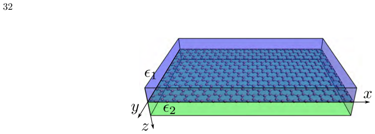
Dispersion relation — transverse magnetic modes For this derivation, we will closely follow Ref. [47]. We consider a system consisting of a single graphene sheet clad between two semi-infinite dielectric media, characterized by the real dielectric constants (relative permittivi...
-
[13]
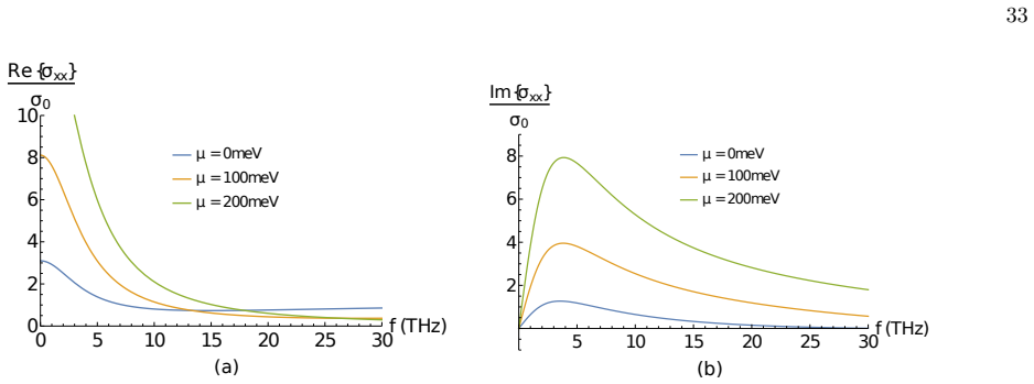
Results for single layer graphene In Fig. 24, we present our results for the total conductivity (Drude plus regular terms) in SLG, as a function of the frequency,f = ω/(2π), across the spectral region where we are interested to study the spectrum of graphene SPPs —from the THz...
-
[14]
27, for two different twist angles
Results for twisted bilayer graphene For the tBLG, we repeat the previous analysis, namely the last 2 plots from Fig. 27, for two different twist angles. We start withθ= 9◦(Fig. 28). For this angle, we see that the signature of the curves do not differ a lot from those of the SL...
2020
-
[15]
A. K. Geim. Graphene: status and prospects.Science, 324(5934):1530–1534, 2009
2009
-
[16]
S. Z. Butler, S. M. Hollen, L. Cao, Y. Cui, J. A. Gupta, H. R. Gutiérrez, T. F. Heinz, S. S. Hong, J. Huang, A. F. Ismach, E. Jonhston-Halperin, M. Kuno, V. V. Plashnitsa, R. D. Robinson, R. S. Ruoff, S. Salahuddin, J. San, L. Shi, M. G. Spencer, M. Terrones, W. Windl, J. E. Go...
2013
-
[17]
S. Das, J. A. Robinson, M. Dubey, H. Terrones, M. Terrones. Beyond graphene: progress in novel two-dimensional materials and van der Waals solids.Annu. Rev. Mater. Res., 45:1–27, 2015
2015
-
[18]
K. S. Novoselov, A. H. C. Neto. Two-dimensional crystals-based heterostructures: materials with tailored properties.Phys. Scr., T146:014006, 2012
2012
-
[19]
K. S. Novoselov, A. Mishchenko, A. Carvalho, A. H. C. Neto. 2D materials and van der Waals heterostructures.Science, 353(6298):aac9439, 2016
2016
-
[20]
J. M. B. Lopes dos Santos, N. M. R. Peres, A. H. C. Neto. Continuum model of the twisted graphene bilayer.Phys. Rev. B, 86(15):155449, 2012. 37
2012
-
[21]
Brihuega, P
I. Brihuega, P. Mallet, H. González-Herrero, G. Trambly de Laissardière, M. M. Ugeda, L. Magaud, J.M. Gómez-Rodríguez, F.Ynduráin, J.-Y.Veuillen. UnravellingtheintrinsicandrobustnatureofvanHovesingularitiesintwistedbilayergraphene. Phys. Rev. Lett., 109(19):196802, 2012
2012
-
[22]
Latil, V
S. Latil, V. Meunier, L. Henrard. Massless fermions in multilayer graphitic systems with misoriented layers: ab initio calculations and experimental fingerprints.Phys. Rev. B, 76(20):201402, 2007
2007
-
[23]
E. S. Morell, J. D. Correa, P. Vargas, M. Pacheco, Z. Barticevic. Flat bands in slightly twisted bilayer graphene: tight- binding calculations. Phys. Rev. B, 82(12):121407, 2010
2010
-
[24]
G. T. de Laissardière, D. Mayou, L. Magaud. Numerical studies of confined states in rotated bilayer of graphene.Phys. Rev., 86(12):125413, 2012
2012
-
[25]
J. M. B. Lopes dos Santos, N. M. R. Peres, A. H. C. Neto. Graphene bilayer with a twist: electronic structure.Phys. Rev. Lett., 99(25):256802, 2007
2007
-
[26]
Bistritzer, A
R. Bistritzer, A. H. MacDonald. Moiré bands in twisted double-layer graphene.PNAS, 108(30):12233–12237, 2011
2011
-
[27]
de Gail, M
R. de Gail, M. O. Goerbig, F. Guinea, G. Montambaux, A. H. C. Neto. Topologically protected zero modes in twisted bilayer graphene.Phys. Rev. B, 84(4):045436, 2011
2011
-
[28]
Interlayer interaction in general incommensurate atomic layers.New Journal of Physics, 17(1):015014, 2015
Mikito Koshino. Interlayer interaction in general incommensurate atomic layers.New Journal of Physics, 17(1):015014, 2015
2015
-
[29]
Weckbecker, S
D. Weckbecker, S. Shallcross, M. Fleischmann, N. Ray, S. Sharma, O. Pankratov. Low-energy theory for the graphene twist bilayer.Phys. Rev. B, 93(3):035452, 2016
2016
-
[30]
A. K. Geim, A. H. MacDonald. Graphene: exploring carbon flatland.Phys. Today, 60(8):35–41, 2007
2007
-
[31]
A. H. C.Neto, F. Guinea, N. M. R. Peres, K. S. Novoselov, A. K. Geim. The electronic properties of graphene.Rev. Mod. Phys., 81(1):109, 2009
2009
-
[32]
Reich, J
S. Reich, J. Maultzsch, C. Thomsen. Tight-binding description of graphene.Phys. Rev. B, 66(3):035412, 2002
2002
-
[33]
C. Bena, G. Montambaux. Remarks on the tight-binding model of graphene.New J. Phys., 11(9):095003, 2009
2009
-
[34]
Thermal transport for many-body tight-binding models.Phys
Indranil Paul, Gabriel Kotliar. Thermal transport for many-body tight-binding models.Phys. Rev. B, 67:115131, Mar 2003
2003
-
[35]
D. K. Efetov, P. Kim. Controlling electron-phonon interactions in graphene at ultrahigh carrier densities.Phys. Rev. Lett., 105(25):256805, 2010
2010
-
[36]
A. Das, S. Pisana, B. Chakraborty, S. Piscanec, S. K. Saha, U. V. Waghmare, K. S. Novoselov, H. R. Krishnamurthy, A. K. Geim, A. C. Ferrari, A. K. Sood. Monitoring dopants by Raman scattering in an electrochemically top-gated graphene transistor. Nature nanotechnology, 3(4):21...
2008
-
[37]
K. F. Mak, C. H. Lui, J. Shan, T. F. Heinz. Observation of an electric-field-induced band gap in bilayer graphene by infrared spectroscopy.Phys. Rev. Lett., 102(25):256405, 2009
2009
-
[38]
Fleck, AN
M. Fleck, AN. M. Oleś, L. Hedin. Magnetic phases near the van Hove singularity in s-and d-band Hubbard models.Phys. Rev. B, 56(6):3159, 1997
1997
-
[39]
González
J. González. Kohn-Luttinger superconductivity in graphene.Phys. Rev. B, 78(20):205431, 2008
2008
-
[40]
Nandkishore, L
R. Nandkishore, L. S. Levitov, A. V. Chubukov. Chiral superconductivity from repulsive interactions in doped graphene. Nature Physics, 8(2):158–163, 2012
2012
-
[41]
G. Li, A. Luican, J. M. B. Lopes dos Santos, A. H. Castro Neto, A. Reina, J. Kong, E. Y. Andrei. Observation of van Hove singularities in twisted graphene layers.Nature Physics, 6(2):109–113, 2010
2010
-
[42]
A. V. Rozhkov, A. O. Sboychakov, A. I. Rakhmanov, F. Nori. Electronic properties of graphene-based bilayer systems. Physics Reports, 648:1–104, 2016
2016
-
[43]
Gutiérrez-Rubio, Mauricio Sturla, Francisco Guinea
Pablo San-Jose, A. Gutiérrez-Rubio, Mauricio Sturla, Francisco Guinea. Spontaneous strains and gap in graphene on boron nitride. Phys. Rev. B, 90:075428, Aug 2014
2014
-
[44]
J. C. Slater, G. F. Koster. Simplified LCAO method for the periodic potential problem.Phys. Rev., 94(6):1498–1524, 1954
1954
-
[45]
Kretinin, G
A. Kretinin, G. L. Yu, R. Jalil, Y. Cao, F. Withers, A. Mishchenko, M. I. Katsnelson, K. S. Novoselov, A. K. Geim, F. Guinea. Quantum capacitance measurements of electron-hole asymmetry and next-nearest-neighbor hopping in graphene. Phys. Rev. B, 88(16):165427, 2013
2013
-
[46]
Y. Wang, Z. Ni, L. Liu, Y. Liu, C. Cong, T. Yu, X. Wang, D. Shen, Z. Shen. Stacking dependent optical conductivity of bilayer graphene.ACS nano, 4(7):4074–4080, 2010
2010
-
[47]
X. Zou, J. Shang, J. Leaw, Z. Luo, L. Luo, C. La o vorakiat, L. Cheng, S. A. Cheong, H. Su, J.-X. Zhu, Y. Liu, K. P. Loh, A. H. C. Neto, T. Yuand E. E. M. Chia. Terahertz conductivity of twisted bilayer graphene.Phys. Rev. Lett., 110(6):067401, 2013
2013
-
[48]
Y. Cao, J. Y. Luo, V. Fatemi, S. Fang, J. D. Sanchez-Yamagishi, K. Watanabe, T. Taniguchi, E. Kaxiras, P. Jarillo- Herrero. Superlattice-induced insulating states and valley-protected orbits in twisted bilayer graphene.Phys. Rev. Lett., 117(11):116804, 2016
2016
-
[49]
Tabert, E.J
C.J. Tabert, E.J. Nicol. Optical conductivity of twisted bilayer graphene.Phys. Rev. B, 87(12):121402, 2013
2013
-
[50]
P. Moon, M. Koshino. Optical absorption in twisted bilayer graphene.Phys. Rev. B, 87(20):205404, 2013
2013
-
[51]
Optical conductivity, Drude weight and plasmons in twisted graphene bilayers
Tobias Stauber, Pablo San-Jose, Luis Brey. Optical conductivity, Drude weight and plasmons in twisted graphene bilayers. New J. Phys., 15(11):113050, 2013
2013
-
[52]
L. Ju, B. Geng, J. Horng, C. Girit, M. Martin, Z. Hao, H. A. Bechtel, X. Liang, A. Zettl, Y. R. Shen, F. Wang. Graphene plasmonics for tunable terahertz metamaterials.Nature nanotechnology, 6(10):630–634, 2011
2011
-
[53]
Jablan, H
M. Jablan, H. Buljan, M. Soljačić. Plasmonics in graphene at infra-red frequencies.Phys. Rev. B, 80(24):245435, 2009
2009
-
[54]
F. H. L. Koppens, D. E. Chand, F. J. G. de Abajo. Graphene plasmonics: a platform for strong light–matter interactions. 38 Nano Lett., 11(8):3370–3377, 2011
2011
-
[55]
X. Luo, T. Qiu, W. Lu, Z. Ni. Plasmons in graphene: recent progress and applications.Materials Science & Engineering, R: Reports, 74(11):351–376, 2013
2013
-
[56]
Vakil, N
A. Vakil, N. Engheta. Transformation optics using graphene.Science, 332(6035):1291–1294, 2011
2011
-
[57]
Z. Fang, Y. Wang, Z. Liu, A. Schlather, P. M. Ajayan, F. H. L. Koppens, P. Nordlander, N. J. Halas. Plasmon-induced doping of graphene.ACS nano, 6(11):10222–10228, 2012
2012
-
[58]
Z. Fei, A. S. Rodin, G. O. Andreev, W. Bao, A. S. McLeod, M. Wagner, L. M. Zhang, Z. Zhao, M. Thiemens ang G. Dominguez, M. M. Fogler, A. H. C. Neto, C. N. Lau, F. Keilmann, D. N. Basov. Gate-tuning of graphene plasmons revealed by infrared nano-imaging.Nature, 487(7405):82–85, 2012
2012
-
[59]
J. Chen, M. Badioli, P. Alonso-González, S. Thongrattanasiri, F. Huth, J. Osmond, M. Spasenović, A. Centeno, A. Pes- quera, P. Godignon, A. Zurutuza, N. Camara, J. G. de Abajo, R. Hillenbrand, F. Koppens. Optical nano-imaging of gate-tuneable graphene plasmons.Nature, 487(7405...
2012
-
[60]
A. N. Grigorenko, M. Polini, K. S. Novoselov. Graphene plasmonics.Nat. Photonics, 6(11):749–758, 2012
2012
-
[61]
P. A. D. Gonçalves, N. M. R. Peres.An introduction to graphene plasmonics. World Scientific Publishing Co. Pte. Ltd., 2016
2016
-
[62]
D. J. Passos, G. B. Ventura, J. M. Viana Parente Lopes, J. M. B. Lopes dos Santos, N. M. R. Peres. Nonlinear optical responses of crystalline systems: results from a velocity gauge analysis.Phys. Rev. B, 97(23):235446, 2018
2018
-
[63]
N. A. Doughty.Lagrangian interaction. Addison-Wesley, 1990
1990
-
[64]
N. W. Ashcroft, N. D. Mermin.Solid state physics. Harcourt College Publishers, 1976
1976
-
[65]
Kittel.Introduction to solid state physics
C. Kittel.Introduction to solid state physics. John Wiley & Sons, 1966
1966
-
[66]
Stauber, N
T. Stauber, N. M. R. Peres, A. K. Geim. The optical conductivity of graphene in the visible region of the spectrum.Phys. Rev. B, 78(8):085432, 2008
2008
-
[67]
Nowick.Crystal properties via group theory
Arthur S. Nowick.Crystal properties via group theory. Cambridge University Press, 1995
1995
-
[68]
Z. Q. Li, E. A. Henriksen, Z. Jiang, Z. Hao, M. C. Martin, P. Kim, H. L. Stormer, D. N. Basov. Dirac charge dynamics in graphene by infrared spectroscopy.Nature Physics, 4(7):532–535, 2008
2008
-
[69]
S. V. Morozov, K. S. Novoselov, M. I. Katsnelson, F. Schedin, D. C. Elias, J. A. Jaszczak, A. K. Geim. Giant intrinsic carrier mobilities in graphene and its bilayer.Phys. Rev. Lett., 100(1):016602, 2008
2008
-
[70]
A. K. Geim, K. S. Novoselov. The rise of graphene.Nat. Mater., 6(3):183–191, 2007
2007
-
[71]
Eduardo J. C. Dias. Plasmonic effects in unidimensional structures and graphene-based nanostructures. Praca magisterska, Universidade do Minho, Nov 2016
2016
-
[72]
Y. V. Bludov, A. Ferreira, N. M. R. Peres, M. I. Vasilevskiy. A primer on surface plasmon-polaritons in graphene.Int. J. Mod. Phys. B, 27(10):1341001, 2013
2013
-
[73]
Tomarken, Jason Y
Yuan Cao, Valla Fatemi, Ahmet Demir, Shiang Fang, Spencer L. Tomarken, Jason Y. Luo, Javier D. Sanchez-Yamagishi, Kenji Watanabe, Takashi Taniguchi, Efthimios Kaxiras, Ray C. Ashoori, Pablo Jarillo-Herrero. Correlated insulator behaviour at half-filling in magic-angle graphene ...
2018
-
[74]
Unconventional superconductivity in magic-angle graphene superlattices
Yuan Cao, Valla Fatemi, Shiang Fang, Kenji Watanabe, Takashi Taniguchi, Efthimios Kaxiras, Pablo Jarillo-Herrero. Unconventional superconductivity in magic-angle graphene superlattices
Reviewed August 14, 2026 · model on record in the stance chip above.
Discussion (0). Continue with ORCID to comment.