REVIEW 3 major objections 5 minor 37 references
New results in solar modulation modeling in light of recent cosmic-ray data from space
T0 review · 3 major / 5 minor · reviewed 2026-08-14 · deepseek-v4-flash
Pith's one-line read This paper claims that heliospheric cosmic-ray diffusion is time-dependent, extracting from ten years of proton data a normalization $K_0$ that anti-correlates with solar activity and spectral indices $a,b$ that vary over the cycle.
desk verdict A solid, compact fitting study: K0 tracking solar activity is convincing, but the a(t) and b(t) claim needs a constant-parameter null test before it lands. read the letter →
The pith
A machine-rendered reading of the paper's core claim, the machinery that carries it, and where it could break.
The reading
What carries the argument
Central machinery is the Parker–Krymsky transport equation for cosmic-ray phase-space density, solved in steady state with a stochastic backward Monte Carlo method in a spherical heliosphere (termination shock at 85 AU, heliopause at 122 AU). Diffusion enters through a parallel coefficient with a double power law in rigidity: $$K_{\parallel} = \frac{K_0}{3}\$\beta$\left(\frac{B_0}{B}\right)\left(\frac{R_0}{R}\right)^{a}\left[\frac{(R/R_0)^h + (R_k/R_0)^h}{1 + (R_k/R_0)^h}\right]^{\frac{b-a}{h}},$$ with $K_0$ the overall normalization, $a$ and $b$ the low- and high-rigidity spectral indices, $R_k$ the break rigidity, and $h$ the transition smoothness. The argument works by fixing tilt angle, field magnitude, and polarity from solar observations, building a grid of model spectra over $K_0$, $a$, and $b$, and producing best-fit time series from proton data. The key move is that the grid is evaluated for each epoch, making the diffusion parameters themselves the fitted quantities rather than assumed constants.
What would settle it
Refit the 2007–2016 AMS-02 and PAMELA proton time series with an alternative published local interstellar proton spectrum that still matches the Voyager-1 and AMS-02 anchors, and compare the extracted $a(t)$ and $b(t)$: if the temporal trends vanish or invert, they are artifacts of the assumed boundary condition rather than properties of the heliospheric diffusion tensor.
Extended reading notes
Core claim
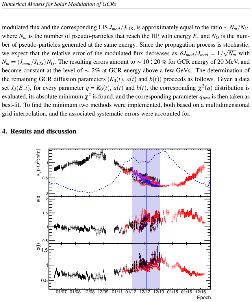
The central claim is that the diffusion tensor governing heliospheric cosmic-ray transport is not a fixed property of the plasma but evolves with the solar cycle. Fitting a stochastic Parker-transport model to time-resolved AMS-02 and PAMELA proton spectra from 2007 to 2016, the authors extract time series for the diffusion normalization $K_0$ and the rigidity spectral indices $a$ and $b$. They report that $K_0$ is well anti-correlated with the smoothed sunspot number, so diffusion is faster at solar minimum and slower at maximum, and that $a$ and $b$ show a clear temporal dependence. The fitted indices agree with the measured slopes of the heliospheric magnetic turbulence spectrum in its $1/f$ and inertial ranges, and the behavior across the 2012–2013 polarity reversal is shown under both field polarities with a modeled smooth transition. On the paper's own argument, constant-diffusion modulation models are insufficient: $K_0$, $a$, and $b$ must be treated as time dependent.
Load-bearing premise
The whole extraction rests on assuming the proton spectrum at the heliopause—taken from earlier fits to Voyager-1 and AMS-02 data—is correct; a biased boundary spectrum would leak into the fitted diffusion parameters and could fake a solar-cycle trend.
Editorial extensions
If this is right
- Time-dependent modulation models must replace the fixed diffusion parameters used in most earlier work; fixed-parameter fits will mis-track the measured spectra near solar maximum and minimum.
- The $K_0(t)$ series provides a transport-level translation of the sunspot cycle, with faster diffusion at minimum and slower diffusion at maximum.
- Variations in $a$ and $b$ imply that the rigidity dependence of diffusion—not just its overall level—changes across the cycle, which affects the shape of the modulated spectrum.
- The agreement of the fitted indices with measured turbulence slopes ties the model to in-situ magnetic-field observations, so future turbulence measurements can be compared directly with the fitted parameters.
- The treatment across the 2012–2013 polarity reversal shows how the fits behave when drift patterns flip, providing a test of drift-dominated modulation during an unstable HMF polarity phase.
Reading between the lines
- Beyond the paper: if the spectral indices $a$ and $b$ truly vary, then propagation codes that keep them constant will bias reconstructed interstellar spectra at low rigidity; rerunning the same fits on helium or on electrons could show whether the trend is charge-sign dependent.
- Beyond the paper: the clean anti-correlation between $K_0$ and the smoothed sunspot number points to a forecasting route—map a solar activity proxy onto transport coefficients and predict future modulated spectra—though the paper does not build such a predictor itself.
- Beyond the paper: a decisive robustness test the paper does not perform is to repeat the extraction with alternative local interstellar spectra; if the $a(t)$ and $b(t)$ trends survive that replacement, the time dependence is a genuine feature of the heliospheric turbulence spectrum.
Signed reviews
Editorial analysis
A structured set of objections, weighed in public.
Referee Report
Summary. This conference proceeding presents a two-dimensional steady-state solar modulation model, solved with a stochastic approach (Solarprop), and uses time-resolved proton data from AMS-02 and PAMELA over 2007–2016 to extract best-fit values of the diffusion normalization K0 and the spectral indices a and b of the parallel diffusion coefficient at successive epochs. The tilt angle, magnetic field intensity, and polarity are taken from solar observations, while the proton local interstellar spectrum (LIS) is adopted from the authors' previous works. The paper reports that K0 is anti-correlated with the smoothed sunspot number and that a and b show clear temporal dependence, implying that the heliospheric diffusion tensor and turbulence spectrum vary over the solar cycle.
Significance. If the reported temporal dependence of K0, a, and b is established, the result is significant for solar modulation physics and for the interpretation of cosmic-ray data in terms of heliospheric turbulence: it would require time-dependent diffusion tensors in modulation models and would connect GCR transport to evolving solar-wind turbulence. The paper has clear strengths: the use of a standard Parker transport equation, a transparent chi-square minimization with Monte Carlo and LIS uncertainties folded into the errors, comparison with public space-borne data, and explicit framing of the extracted parameters as testable time series. However, the central claim is not yet demonstrated because the time dependence is inferred from independent per-epoch fits without a quantitative test against a constant-parameter null model, and because the adopted LIS is fixed without sensitivity tests.
major comments (3)
- [Section 3, Eq. (3.1)] The paper does not test the null hypothesis that K0, a, and b are constant over 2007–2016, with only alpha(t), B0(t), and A(t) allowed to vary. Because the three diffusion parameters in Eq. (2.3) are mutually degenerate over the limited rigidity range of the AMS-02 and PAMELA proton data, the per-epoch best-fit time series in Fig. 2 could absorb the modulation cycle even if the underlying diffusion parameters are constant. The authors should quantitatively compare the time-dependent fit against a constant-parameter model, for example through the chi-square difference or an information criterion, and report whether the temporal variation is statistically required.
- [Section 2 (LIS paragraph)] The proton LIS from refs. [23–25] is used as a fixed boundary condition at the heliopause, and the paper does not test how the extracted time series of K0, a, and b respond to alternative LIS choices. Since that LIS is calibrated partly with AMS-02 high-energy data and Voyager-1 low-energy data, a systematic LIS bias could propagate into a time-dependent bias in the fitted modulation parameters. The authors should perform a sensitivity scan over LIS variations within the stated uncertainties and show that the temporal trends in K0, a, and b survive, or quantify the resulting systematic errors.
- [Section 4, Fig. 2] No comparison between the best-fit model spectra and the measured proton spectra is shown, and no chi-square values, residuals, or uncertainty bands for the fits are reported. Without such a comparison, the reader cannot assess whether the per-epoch fits actually describe the data or whether the parameter time dependence compensates for structural model deficiencies. The authors should show model spectra overlaid on the data and/or residual time series for representative epochs such as solar minimum, maximum, and reversal.
minor comments (5)
- [Abstract] The phrase 'measured-validated model' is awkward; consider 'measurement-validated' or 'data-validated'.
- [Fig. 2 caption] The caption uses 'Tinv' while the text defines 'Trev'; unify the notation and explicitly identify the line types and colors for the SSN curve and the polarity-transition curves.
- [Acknowledgments] The 'Wilkox Solar Observatory' is a typo; it should be 'Wilcox Solar Observatory'.
- [References] Reference [5] lists the article number as '0511012'; this appears to be a typo for '051101'.
- [Section 4] The text states that the smoothed SSN is shown as a dotted blue line, but the figure caption does not state this; please add the SSN curve description to the caption for clarity.
Circularity Check
No significant circularity; the temporal parameter variations are reported as best-fit results, not predictions, and the LIS boundary condition is independently constrained by Voyager-1 and AMS-02 data.
full rationale
The paper's inference of K0(t), a(t), and b(t) is a parameter-estimation exercise: Section 3 describes fitting these three diffusion parameters to epoch-binned AMS-02 and PAMELA proton spectra by minimizing a chi-square statistic, and Section 4 reports the resulting best-fit time series. Because the paper presents these as fitted values rather than as predictions of an independent quantity, there is no reduction of a prediction to a fit input by construction. The boundary LIS is taken from prior works by the authors and collaborators, but those calculations are calibrated against Voyager-1 low-energy data and AMS-02 high-energy data, the paper states that the LIS 'agrees fairly well with other spectra proposed recently,' and the LIS serves only as a boundary condition, not as the quantity whose temporal dependence is claimed. The lack of a quantitative comparison against a time-independent null model and the limited discussion of parameter degeneracy are statistical robustness concerns, not evidence of circular reasoning. No step in the derivation chain equates an output to an input by definition or via a self-citation chain. Therefore the circularity score is 0.
Assumptions & free parameters
free parameters (6)
- K0(t), diffusion normalization =
Time series in Fig. 2, roughly (0.3-1.2) x 10^23 cm^2/s
- a(t), low-rigidity spectral index =
Time series in Fig. 2, roughly 0.6-1.5
- b(t), high-rigidity spectral index =
Time series in Fig. 2, roughly 0.5-1.5
- alpha(t), HCS tilt angle =
Time series from Wilcox Solar Observatory
- B0(t), HMF intensity at Earth =
Time series from Wilcox Solar Observatory
- A(t), HMF polarity =
Plus or minus one, from solar polarity observations
assumptions (6)
- domain assumption The Parker-Krymsky transport equation (Eq. 2.1) with a diffusion-drift model, solved in steady state, describes GCR flux in the heliosphere.
- domain assumption Time dependence is represented as a sequence of steady-state solutions with model inputs averaged over a 12-month window.
- domain assumption The proton LIS used as boundary condition at the heliopause is correct.
- domain assumption Parallel diffusion follows the double power law of Eq. 2.3 with fixed break rigidity Rk and smoothness h; perpendicular diffusion is xi = 0.02 times parallel with polar corrections.
- domain assumption The heliosphere can be modeled as a spherical cavity with termination shock at 85 AU and heliopause at 122 AU, with solar wind speed from the parameterization of ref. [14].
- standard math The chi-square statistic with sigma^2 = sigma_d^2 + sigma_mod^2 correctly captures experimental, Monte Carlo, and LIS uncertainties.
Cite this review
Pith. "Pith review of New results in solar modulation modeling in light of recent cosmic-ray data from space." pith.science (2026). https://pith.science/paper/CIHJFWS7
@misc{pith2026190801599,
  author       = {Pith},
  title        = {Pith review of: New results in solar modulation modeling in light of recent cosmic-ray data from space},
  year         = {2026},
  howpublished = {\url{https://pith.science/paper/CIHJFWS7}},
  note         = {Machine review of arXiv:1908.01599}
}
read the original abstract
Thanks to space-borne experiments such as the AMS-02 and PAMELA missions in low-Earth orbit, along with the Voyager spacecrafts in the interstellar space, a large collection of multi-channel and time-resolved Galactic cosmic ray (GCR) data has recently become available. Here we present an improved measured-validated model of the "solar modulation" effect, i.e., the temporal evolution of the GCR flux inside the heliosphere caused by the 11-year variability cycle of the Sun's magnetic activity. We present our improved modeling of the structure of the heliosphere, the physical mechanisms of diffusion, drift, and energy losses of GCR particles in the heliosphere. We present our results for the temporal dependence of the key model parameters and their relationship with solar activity proxies. We discuss implications for the GCR transport in magnetic turbulence, and new insights on our understanding of the solar modulation phenomenon.
Figures

Reference graph
Works this paper leans on
-
[1]
Usoskin, I.G., et al., J. Geophys. Res. 103, 9567 (1998) 6 Numerical Models for Solar Modulation of GCRs
work page 1998
-
[2]
Ross, E., Chaplin, W., Sol. Phys. 294, 8 (2019)
work page 2019
-
[3]
C., et al., Astrophys
Cummings, A. C., et al., Astrophys. J. 831, 18 (2016)
2016
-
[4]
Aguilar, M., et al., Phys. Rev. Lett. 121, 051101 (2018)
2018
-
[5]
Aguilar, M., et al., Phys. Rev. Lett. 121, 0511012 (2018)
work page 2018
-
[6]
Adriani, O., et al., Astrophys. J. 765, 91, (2013)
2013
-
[7]
Martucci, M., et al., Astrophys. J. 854, L2 (2018)
2018
-
[8]
Parker, E. N., Planet. Space Sci. 13, 9 (1965) Krymsky, G., Geomagn. Aéron. 4, 977-987 (1964)
work page 1965
Show all 37 references
-
[9]
S., Living Rev
Potgieter, M. S., Living Rev. Solar Phys., 10, 3 (2013)
2013
-
[10]
176 299 (2013)
Moraal, H., Space Sci Rev. 176 299 (2013)
2013
-
[11]
D., Effenberger, F., Space Sci Rev (2017)
Strauss, R. D., Effenberger, F., Space Sci Rev (2017)
2017
-
[12]
Kappl, R., Comp. Phys. Comm. 207 (2016) 386-399
2016
-
[13]
Tomassetti, N., Phys. Rev. D 96, 103005 (2017)
2017
-
[14]
S., et al., Sol
Potgieter, M. S., et al., Sol. Phys. 289, 391-406 (2014)
2014
-
[15]
T., Space Sci
Hoeksema, J. T., Space Sci. Rev. 72, 137-148 (1995)
1995
-
[16]
G., Mursula, K
Alanko-Huotari, K., Usoskin, I. G., Mursula, K. Kovaltsov, G. A., Adv. Space Res. 40, 1064-1069 (2007)
2007
-
[17]
R., Astrophys
Giacalone, J., & Jokipii, J. R., Astrophys. J. 520, 204 (1999)
1999
-
[18]
H., Osman K
Kiyani K. H., Osman K. T., Chapman S.C., Phil. Trans. R. Soc. A 373: 20140155 (2015)
2015
-
[19]
A., Nuovo Cimento C, 19C, 935-943 (1996)
Simpson, J. A., Nuovo Cimento C, 19C, 935-943 (1996)
1996
-
[20]
Heber, B., et al., J. Geophys. Res., 103, 4809 (1998)
1998
-
[21]
Manuel, R., Ferreira, S. E. S., Potgieter, M. S., Sol. Phys. 289, 2207 (2014)
2014
-
[22]
A., Black, J
Grenier, I. A., Black, J. H., Strong, A. W., Annu. Rev. Astron. Astrophys. 53, 199 (2015)
2015
-
[23]
Tomassetti, N., Phys. Rev. D 92, 081301 (2015); Tomassetti, N. Astrophys. J. Lett. 752, L13 (2012)
2015
-
[24]
Feng, J., Tomassetti, N., Oliva, A., Phys. Rev. D 94, 123007 (2016)
2016
-
[25]
Tomassetti, N., Bertucci, B., Barão, F., et al., Phys. Rev. Lett. 121, 251104 (2018)
2018
-
[26]
Aguilar, M., et al., Phys. Rev. Lett. 114, 171103 (2015)
2015
-
[27]
Aguilar, M., et al., Phys. Rev. Lett. 115, 211101 (2015)
2015
-
[28]
J., et al., Astrophys
Boschini, M. J., et al., Astrophys. J. 840, 115 (2017)
2017
-
[29]
Corti, C., et al., Astrophys. J. 871, 253 (2019)
2019
-
[30]
Corti, C., Bindi, V ., Consolandi, C., Whitman, K., Astrophys. J. 829, 8 (2016)
2016
-
[31]
Tomassetti, N., Orcinha, M., Barão, F., Bertucci, B., Astrophys. J. Lett. 849, 32 (2017)
2017
-
[32]
Tomassetti, N., Astrophys. J. Lett. 815, L1 (2015)
2015
-
[33]
Space Res
Tomassetti, N., Adv. Space Res. 60, 815-825 (2017)
2017
-
[34]
T., Liu, Y ., and Zhao, J.,Astrophys
Sun, X., Hoeksema, J. T., Liu, Y ., and Zhao, J.,Astrophys. J. 798, 114 (2015)
2015
-
[35]
Vaisanen, P., Usoskin, I., Mursula, K., J. Geophys. Res.: Space Phys. 124, 804-811 (2019)
2019
-
[36]
Borovsky, J. E., J. Geophys. Res. 117, A05104 (2012)
2012
-
[37]
S., Forman, M
Horbury, T. S., Forman, M. A., & Oughton, S., Plasma Phys. Contr. Fusion, 47, B703-B717 (2005) 7
2005
Reviewed August 14, 2026 · model on record in the stance chip above.
Discussion (0). Continue with ORCID to comment.