REVIEW 3 major objections 5 minor 15 references
StateSpaceModels.jl: a Julia Package for Time-Series Analysis in a State-Space Framework
T0 review · 3 major / 5 minor · reviewed 2026-08-14 · deepseek-v4-flash
Pith's one-line read StateSpaceModels.jl provides a complete state-space workflow in Julia, from user-defined linear models to forecasting and Monte Carlo simulation.
desk verdict Useful Julia state-space package, but the printed seasonal recursion is explosive — needs a fix before the paper can be trusted. read the letter →
The pith
A machine-rendered reading of the paper's core claim, the machinery that carries it, and where it could break.
The reading
What carries the argument
The central object is the Gaussian state-space model together with its Kalman filter recursion. The model is defined by the observation equation $y_t = Z_t\alpha_t + \varepsilon_t$ and the state equation $\alpha_{t+1} = T\alpha_t + R\eta_t$, with covariance matrices $H_t$ and $Q_t$; the package fixes $T$, $R$, $H$, and $Q$ to be time-invariant while allowing $Z_t$ to vary. The Kalman filter produces predictive states $a_{t+1}=E[\alpha_{t+1}|Y_t]$, filtered states $a_{t|t}=E[\alpha_t|Y_t]$, innovations $v_t=y_t-Z_ta_t$, and innovation covariances $F_t$, which feed the log-likelihood $\ell(Y_n)=-\frac{np}{2}\log 2\pi - \frac12 \sum_t (\log |F_t|+v_t^\top F_t^{-1}v_t)$. The smoother computes $\hat\alpha_t=E[\alpha_t|Y_n]$, and missing observations are treated by setting $Z_t=0$. This machinery carries the package's claims because every advertised operation—estimation, completion of missing data, forecasting, and scenario simulation—is a consequence of these recursions.
What would settle it
Simulate a state-space series, delete observations whenever the latent state crosses a threshold (a non-ignorable missingness mechanism), fit the package's local level model, and compare the smoothed states and forecasts with the full-data estimates; systematic divergence would falsify the automatic missing-data claim.
Extended reading notes
Core claim
The paper establishes that the package realizes a practical implementation of the Gaussian state-space framework: observations $y_t = Z_t\alpha_t + \varepsilon_t$ and states $\alpha_{t+1}=T\alpha_t+R\eta_t$, with $\varepsilon_t\sim N(0,H)$ and $\eta_t\sim N(0,Q)$. The estimation routine runs the Kalman filter within each maximum-likelihood iteration, using the prediction-error decomposition of the log-likelihood, and then applies a smoother to reconstruct the unobserved states. Missing values marked as NaN are handled by setting $Z_t=0$ in those periods, and forecasts are produced by treating future observations as missing. The paper demonstrates the workflow on airline passenger data, electricity consumption with an exogenous temperature series, and a vehicle-tracking problem defined through a user-supplied model.
Load-bearing premise
The load-bearing premise is that setting $Z_t=0$ for periods with NaN yields valid estimates, which holds only when missingness does not depend on the unobserved state—an assumption the paper neither states nor tests.
Editorial extensions
If this is right
- A Julia user can estimate pre-defined local level, linear trend, and structural models with a single function call, and obtain filtered, smoothed, and predicted states.
- Any linear model expressible through constant or time-varying $Z_t$ and constant $T,R$ can be fitted without writing a Kalman filter or optimizer by hand.
- Series with missing periods (NaN) can be estimated and completed; forecasts are obtained by treating the future as missing.
- Monte Carlo simulation produces $N \times S$ matrices of future scenarios, suitable as inputs to stochastic optimization.
- The square-root Kalman filter and pluggable filter and optimization methods give users control over numerical stability and estimation.
Reading between the lines
- The paper's automatic missing-data completion implicitly assumes that missingness is ignorable; if missing values depend on the unobserved state, the completed series and forecasts would be biased—a testable condition the paper does not discuss.
- The multi-seed L-BFGS strategy is a heuristic for nonconvex likelihood surfaces; the paper does not report diagnostics such as Hessian-based standard errors or convergence checks, so users should treat reported log-likelihoods as point estimates.
- The claim of features absent from commercial software is a snapshot at publication time; the durable contribution is the user-defined linear model interface plus simulation, which other tools could copy, so the package's long-term value depends on maintenance and ecosystem integration.
- Because the framework assumes time-invariant $T,R,H,Q$, the package does not cover models with time-varying state dynamics or stochastic volatility; extending it in that direction is a natural next step.
Signed reviews
Editorial analysis
A structured set of objections, weighed in public.
Referee Report
Summary. The manuscript describes StateSpaceModels.jl, an open-source Julia package for Gaussian state-space time-series analysis. It implements the observation and state equations following Durbin and Koopman, a set of pre-defined models (local level, linear trend, basic structural model, and structural model with exogenous variables), Kalman filtering and smoothing including square-root variants, maximum likelihood estimation of noise covariances via L-BFGS with random seeds, automatic missing-data treatment, forecasting, and Monte Carlo simulation. Three applications are presented: log-airline-passenger forecasting and component extraction, electricity-consumption scenario simulation with an exogenous temperature variable, and vehicle tracking with a user-defined linear model. The central claim is that the package fills a gap as a Julia-native state-space toolbox with features such as Monte Carlo simulation and arbitrary user-defined linear models.
Significance. If the technical issues are resolved, this is a useful open-source contribution: it provides a unified Julia interface for model specification, estimation, filtering, smoothing, forecasting, and simulation, and it appears to offer features not found in related commercial software. The paper's strength is that it exposes the full workflow with reproducible example code and links to a public repository. However, the current evidence for correctness is visual and qualitative only; there are no tests, no benchmark comparisons against KFAS, Statsmodels, or STAMP, and no quantitative forecast or estimation metrics. The sign error in the seasonal recursion, Eq. (13), means that the structural-model examples in Sections 6.1 and 6.2 cannot currently be accepted as evidence without clarification or correction.
major comments (3)
- [§3.1.3, Eq. (13)] The seasonal recursion as printed, γ_{t+1} = Σ_{j=1}^{s-1} γ_{t+1-j} + ω_t, is not the standard zero-sum seasonal model and is explosive for s > 2. With s = 3, substituting the recursion into S_{t+1} = γ_{t+1} + γ_t + γ_{t-1} gives S_{t+1} = 2(γ_t + γ_{t-1}) + ω_t rather than ω_t, and the characteristic roots of γ_{t+1} = γ_t + γ_{t-1} are 1.618 and -0.618. The standard Durbin-Koopman recursion has minus signs: γ_{t+1} = -Σ_{j=1}^{s-1} γ_{t+1-j} + ω_t. Since two of the three applications (Sections 6.1 and 6.2) rely on the structural model, the authors must either correct Eq. (13) or, if the package code actually follows the printed plus signs, revise the implementation and rerun the examples. This is a load-bearing correctness issue, not a merely cosmetic typo.
- [§6.3, state-space representation after Eq. (24)] The observation equation is written as y_t = Z_t α_{t+1} + ε_t, which is inconsistent with Eq. (1), where y_t = Z_t α_t + ε_t, and also with the simulation loop in the same section, which evaluates y[t, :] = Z * α[t, :]. Please correct the indexing (either use α_t or explicitly define an offset state convention and relate it to Eq. (1)) and check that the filter and smoother implementation follows the stated convention.
- [§4.4] The automatic missing-data treatment is presented as yielding 'minimum variance linear unbiased estimates' by setting Z_t = 0 for periods containing NaN. This claim is only valid under an ignorable-missingness assumption (MCAR, or MAR when estimation is likelihood-based) for the Gaussian state-space model. The paper does not state this assumption, nor does it describe how y_t, the innovations v_t, and the log-likelihood in Eq. (21) are modified for missing periods (e.g., whether y_t is set to zero and the observation contribution is omitted). Please make the assumption explicit and describe the exact implementation, since non-ignorable missingness would bias the completed series and forecasts.
minor comments (5)
- [§2] There is a phrasing error: 'Note that the we can rewrite this model' should be 'Note that we can rewrite this model'.
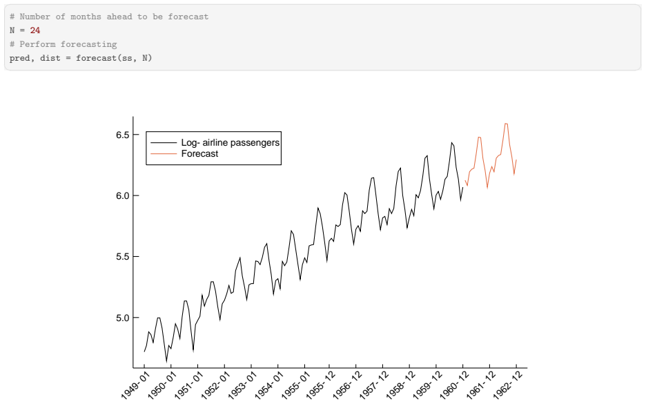
- [§6.1 and §6.2] The application figures are qualitative. Reporting numerical model-selection or forecast-accuracy measures (log-likelihood, AIC, RMSE, or quantile coverage) and, where possible, comparisons with KFAS or Statsmodels on the same data would substantiate the claim that the package is straightforward and functionally complete.
- [§6.2] The statement that the mean of the simulated scenarios is identical to the forecast is correct for a linear Gaussian model when parameters are fixed, but the paper should state explicitly that parameter uncertainty is not propagated in the simulation.
- [§6.3] The code uses variables m and q without definitions in the displayed snippet; adding dimension definitions would make the example self-contained and reproducible.
- [References] Kalman.jl and StateSpace.jl are listed with GitHub links but no version tags or DOIs; for reproducibility, consider citing released versions or specific commits.
Circularity Check
No significant circularity: standard textbook methods implemented and demonstrated; self-citations are not load-bearing.
full rationale
This is a software-description paper, not a paper that derives predictions from fitted parameters. The state-space framework, Kalman filter, maximum likelihood estimation, and smoothing are imported from the standard external reference [4] (Durbin and Koopman), and the package implements those textbook recursions. The applications in Section 6 are demonstrations of the software rather than scientific claims whose outputs are forced by their inputs: the airline and electricity examples use a structural model estimated on historical data and then show forecasts or simulations, which is normal out-of-sample use, not a fitted parameter being renamed as a prediction. The vehicle-tracking example simulates data from known state-space equations and then filters them, which is a self-contained software check rather than a circular derivation. The only self-citations are [11], which points to the package repository, and [15], which cites the authors' earlier energy-demand study as related work; neither is load-bearing for the mathematical content of the paper. The paper does contain a likely sign error in Eq. (13), where the printed seasonal recursion with plus signs would not deliver the stated zero-sum seasonality property; however, a sign typo is a correctness risk, not circularity, because the claimed property does not reduce to the printed equation by construction. Overall, no step in the paper's argument is equivalent to its own inputs, so the circularity score is 0.
Assumptions & free parameters
assumptions (4)
- domain assumption Observations follow the Gaussian state-space equations y_t = Z_t alpha_t + epsilon_t, alpha_{t+1} = T_t alpha_t + R_t eta_t, with independent Gaussian noises (Section 2).
- standard math The Kalman filter and smoother recursions referenced from Durbin and Koopman are correct and numerically stable in the standard and square-root variants (Sections 4.1 and 4.3).
- standard math The Gaussian log-likelihood in Eq. (21), computed from innovations, is the correct objective for maximum likelihood estimation of H and Q (Section 4.2).
- domain assumption RandomSeedsLBFGS finds a satisfactory optimum of the log-likelihood (Section 4.2).
Cite this review
Pith. "Pith review of StateSpaceModels.jl: a Julia Package for Time-Series Analysis in a State-Space Framework." pith.science (2026). https://pith.science/paper/XUIY3U7Q
@misc{pith2026190801757,
  author       = {Pith},
  title        = {Pith review of: StateSpaceModels.jl: a Julia Package for Time-Series Analysis in a State-Space Framework},
  year         = {2026},
  howpublished = {\url{https://pith.science/paper/XUIY3U7Q}},
  note         = {Machine review of arXiv:1908.01757}
}
read the original abstract
StateSpaceModels.jl is an open-source Julia package for modeling, forecasting and simulating time series in a state-space framework. The package represents a straightforward tool that can be useful for a wide range of applications that deal with time series. In addition, it contains features that are not present in related commercial software, such as Monte Carlo simulation and the possibility of setting any user-defined linear model.
Figures


Figures from the paper (2 more)


Reference graph
Works this paper leans on
-
[1]
L. Zadeh and C. Desoer,Linear System Theory: The State Space Approach . Courier Dover Publi- cations, 2008
work page 2008
-
[2]
A new approach to linear filtering and prediction problems,
R. E. Kalman, “A new approach to linear filtering and prediction problems,”Journal of Basic Engineering, vol. 82, no. 1, pp. 35–45, 1960
work page 1960
-
[3]
An introduction to the Kalman filter,
G. Welch, G. Bishopet al., “An introduction to the Kalman filter,” Department of Computer Science, University of North Carolina at Chapel Hill, Tech. Rep., 1995
work page 1995
-
[4]
J. Durbin and S. J. Koopman,Time Series Analysis by State Space Methods . Oxford University Press, 2012. 13
work page 2012
-
[5]
KFAS: Exponential family state space models in R,
J. Helske, “KFAS: Exponential family state space models in R,”Journal of Statistical Software , vol. 78, no. 10, pp. 1–39, 2017
work page 2017
-
[6]
Statsmodels: Econometric and statistical modeling with Python,
S. Seabold and J. Perktold, “Statsmodels: Econometric and statistical modeling with Python,” in 9th Python in Science Conference , 2010
work page 2010
-
[7]
STAMP 6.0: Structural time series analyser, modeller and predictor,
S. J. Koopman, A. C. Harvey, J. A. Doornik, and N. Shephard, “STAMP 6.0: Structural time series analyser, modeller and predictor,”London: Timberlake Consultants , 2000
work page 2000
-
[8]
M. Schauer, “Kalman.jl,” [Online]. Available: https://github.com/mschauer/Kalman.jl
Show all 15 references
-
[9]
StateSpace.jl,
“StateSpace.jl,” [Online]. Available: https://github.com/ElOceanografo/StateSpace.jl
-
[10]
ControlSystems.jl: A Control Systems Toolbox for Julia,
F. B. Carlson and M. Fält, “ControlSystems.jl: A Control Systems Toolbox for Julia,” 2016 [Online]. Available: https://github.com/JuliaControl/ControlSystems.jl
2016
-
[11]
StateSpaceModels.jl,
R. Saavedra, G. Bodin, and M. Souto, “StateSpaceModels.jl,” [Online]. Available: https://github. com/LAMPSPUC/StateSpaceModels.jl
-
[12]
Casella and R
G. Casella and R. L. Berger,Statistical Inference. Duxbury Pacific Grove, CA, 2002, vol. 2
2002
-
[13]
On the limited memory BFGS method for large scale optimization,
D. C. Liu and J. Nocedal, “On the limited memory BFGS method for large scale optimization,” Mathematical programming, vol. 45, no. 1-3, pp. 503–528, 1989
1989
-
[14]
Optim: A mathematical optimization package for Julia,
P. K. Mogensen and A. N. Riseth, “Optim: A mathematical optimization package for Julia,”Journal of Open Source Software , vol. 3, no. 24, 2018
2018
-
[15]
Simulating low and high-frequency energy demand scenarios in a unified framework–Part I: Low-frequency simulation,
R. Saavedra, G. Bodin et al. , “Simulating low and high-frequency energy demand scenarios in a unified framework–Part I: Low-frequency simulation,” inProceedings of the L Simpósio Brasileiro de Pesquisa Operacional, 2018. 14
2018
Reviewed August 14, 2026 · model on record in the stance chip above.
Discussion (0). Continue with ORCID to comment.