REVIEW 2 major objections 6 minor 43 references
An efficient, open source, iterative ISPH scheme
T0 review · 2 major / 6 minor · reviewed 2026-08-14 · deepseek-v4-flash
Pith's one-line read The paper claims that the pressure-Poisson equation in incompressible smoothed particle hydrodynamics can be solved by a simple iterative Jacobi/SOR scheme instead of a sparse linear solver, and that this change makes ISPH fast and easy…
desk verdict A reproducible, practical ISPH method with credible benchmarks, but the efficiency claim rests on an unverified stopping criterion and the cylinder comparison needs a baseline. read the letter →
The pith
A machine-rendered reading of the paper's core claim, the machinery that carries it, and where it could break.
The reading
What carries the argument
The load-bearing object is the iterative rewrite of the discretized pressure-Poisson equation (17) into the SOR update (28): $p^{k+1}_i = \omega \left(\mathrm{RHS}_i - \sum_j \mathrm{OD}_{ij} p^k_j\right)/D_{ii} + (1-\omega) p^k_i$, with convergence monitored by the relative-change criterion (29). This turns the sparse solve into a per-particle accumulation, which is trivially parallelized; the scheme's other components — the GTVF background-pressure force (15) for homogeneity, and the Shepard-interpolated wall pressure with position-only normals (41)-(42) — keep particles uniform and boundaries leakage-free so the iteration stays stable at larger timesteps.
What would settle it
Measure the average number of pressure iterations per timestep as particle count N and Reynolds number grow on a stiff benchmark (e.g., lid-driven cavity at Re=10000 or flow past a cylinder at Re=200 with an order-of-magnitude finer resolution). If iteration counts grow appreciably with N or Re rather than staying in the 2-10 range, the claimed speed advantage over the sparse solver — and the simplicity of the GPU implementation — would disappear.
Extended reading notes
Core claim
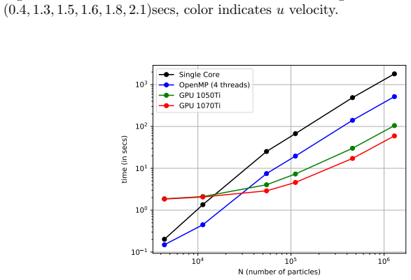
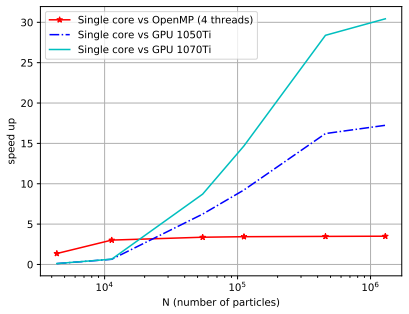
The central claim is that a matrix-free, iteratively solved pressure-Poisson equation — equation (28) with omega=0.5 and tolerance 0.01 — together with GTVF-based particle regularization and a modified dummy-particle wall condition, delivers a generally applicable, accurate ISPH scheme. Whereas conventional ISPH assembles a sparse matrix and solves it with BiCGStab or similar, the new scheme rewrites the PPE as a diagonal-plus-off-diagonal iteration that needs only one scalar accumulation per particle, so the whole method runs with the same ease as weakly-compressible SPH. Benchmarks show accuracy matching matrix-based ISPH with shifting, stability where single-iteration EISPH fails at Re=10000, and an order-of-magnitude speedup at large particle counts, plus linear scaling on GPUs.
Load-bearing premise
The scheme is efficient only if the Jacobi/SOR pressure iteration converges in a small number of iterations per timestep; the paper documents that for a cavity and a dam break, but not for the full range of problems it claims.
Editorial extensions
If this is right
- ISPH implementations no longer need a sparse linear solver; the pressure solve becomes a per-particle accumulation that maps directly onto GPU kernels.
- The scheme should scale to larger 3D problems than typical matrix-based ISPH because only three scalar values per particle are stored for the pressure solve.
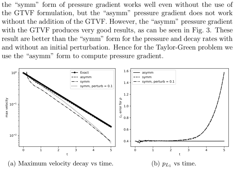
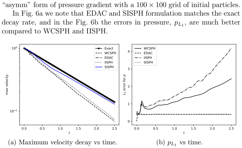
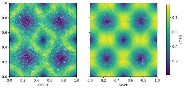
- Single-iteration EISPH is insufficient at high Reynolds numbers; iterating the same PPE to a tolerance around 0.01 stabilizes Taylor-Green at Re=10000.
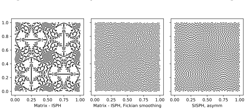
- The GTVF regularization, applied in sub-steps, replaces tuned particle-shifting algorithms and keeps particle distributions homogeneous for internal and free-surface flows.
- Modified dummy-particle wall conditions with position-only normals allow WCSPH-style solid boundaries to be used in ISPH without leakage.
Reading between the lines
- The same matrix-free iterative approach could be applied to other projection methods whose pressure solve dominates cost, such as incompressible Euler or fluid-structure interaction, whenever GPU simplicity is valued over per-iteration convergence rate.
- A natural testable extension is to make the tolerance (or the SOR relaxation omega) adaptive — e.g., tied to the local truncation error O(h^2) — which could keep iteration counts uniform across resolutions and Reynolds numbers.
- The slip/no-slip choice for the intermediate velocity field suggests that the boundary treatment of u* is as important as the pressure solve itself at high Reynolds numbers; a systematic study of that choice could further improve noise and accuracy.
- If iteration counts stay bounded, Jacobi/SOR may beat Krylov solvers on GPUs even when Krylov converges in fewer iterations, because the per-iteration cost and memory traffic are much lower.
Signed reviews
Editorial analysis
A structured set of objections, weighed in public.
Referee Report
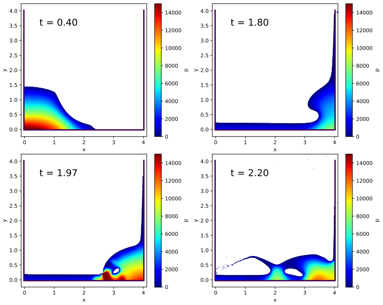
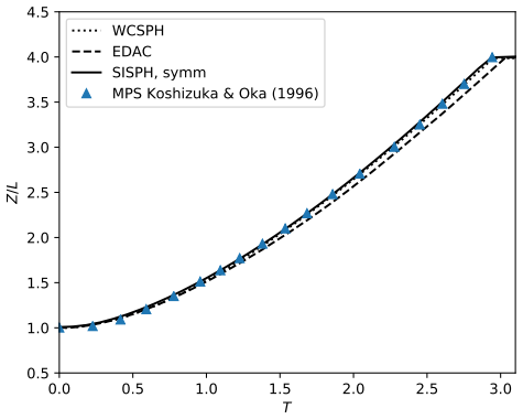
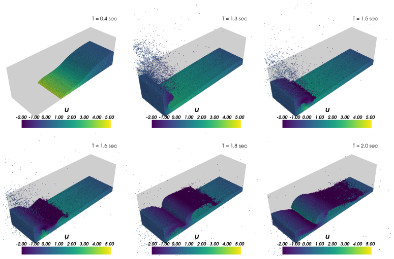
Summary. This paper proposes an iterative, matrix-free formulation of the projection-based ISPH scheme of Cummins and Rudman. The pressure-Poisson equation (17) is solved with an under-relaxed Jacobi/SOR iteration (28) using a change-based stopping criterion (29), eliminating the need to assemble and solve a sparse linear system. Particle ordering is controlled by a generalized transport-velocity formulation (GTVF) with a background pressure, and solid boundaries are treated with a modified Adami-type dummy-particle condition. The method is implemented in the open-source PySPH framework and demonstrated on Taylor-Green vortices, lid-driven cavities at Re=100 and 10000, a square patch, 2D and 3D dam breaks, and flow past a circular cylinder at Re=200, with CPU and GPU performance studies. The central claims are that the scheme is accurate, efficient, easy to implement on GPUs, and requires no sparse linear solvers.
Significance. If the claims hold, the paper provides a practical simplification of ISPH: a matrix-free pressure solve that is straightforward to parallelize on GPUs, combined with GTVF regularization and a wall treatment that works at ISPH timesteps. The strengths of the manuscript are its open-source, reproducible implementation; validation of velocity fields against the exact Taylor-Green solution and the Ghia et al. cavity data; and a 3D dam-break GPU benchmark with scaling data. The paper also honestly demonstrates that a single explicit PPE iteration (EISPH) is inadequate at Re=10000, which motivates the iterative strategy. However, the central efficiency claim currently rests on an unverified stopping criterion, and the cylinder force coefficients are not compared with reference data, so the accuracy claim for external flows is only partially supported.
major comments (2)
- [§3, Eqs. (28)–(29), Table 1] The stopping criterion (29) is based on the relative change in the pressure iterate, not on the residual of the discrete pressure-Poisson equation (17). Since the update (28) with omega=0.5 is a damped Jacobi step, the change ||p^{k+1}-p^k|| is scaled by omega=0.5 regardless of whether the fixed point has been reached, and the denominator max(Lambda, sum|p^{k+1}|) can be large when the mean pressure is large. Moreover, with the minimum of two iterations enforced (Algorithm 1 and Listing 1), the average of 2.0 iterations reported in Table 1 for the cavity at epsilon=0.01 implies the solver almost always exits after the mandatory minimum, not after satisfying (29) in a meaningful way. The paper therefore does not demonstrate that the stopped pressure solves (17) to any useful tolerance, and the claim in Section 3.1 that only a few iterations are necessary is not established. The authors should add a direct convergence check: report the residual norm of (17) at the stopping point for representative cases (lid-driven cavity at Re=100 and Re=10000, and the cylinder), and compare the change-based criterion with a residual-based criterion. This is load-bearing for both the accuracy and efficiency claims.
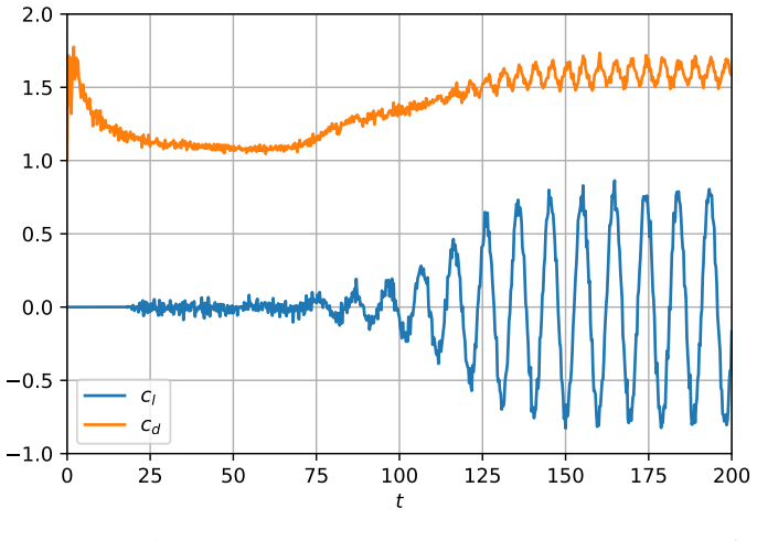
- [§4.7, Fig. 21] The quantitative results of the cylinder benchmark, average cd=1.609 and maximum cl=0.804, are presented without comparison to reference values. The text says the pressure and velocity contours "show an excellent match" with Refs. [38,39], but no force coefficients or Strouhal number from those references are quoted. For unconfined flow past a circular cylinder at Re=200, commonly reported values are around cd≈1.3 and |cl|max≈0.7, so the reported drag is substantially higher and the claimed accuracy is not self-evident. Since this benchmark exercises the modified wall boundary condition and the inlet/outlet treatment, the paper should provide a quantitative comparison (mean drag, peak lift, Strouhal number) against the cited references or other canonical data, and discuss any discrepancy.
minor comments (6)
- [§4.7] The text says "In Fig. 16, we plot the velocity and pressure contour" but this should refer to Fig. 20; Fig. 16 shows the 3D dam break.
- [Eqs. (26)–(27)] The denominator is written as |r_ij|^2 + eta^2, which is inconsistent with Eq. (17) and Listing 2, where the term is |r_ij|^2 + eta h_ij^2; please harmonize the notation.
- [§3] The method in Eq. (28) is damped Jacobi iteration, not successive over-relaxation (SOR), which would require omega>1 and a Gauss-Seidel-type sweep; please correct the terminology.
- [Algorithm 1, lines 13–18] Step 17 computes the final GTVF transport velocity from r^K but appears inside the while loop over k; based on the description in §2.2, it should be executed after the loop terminates.
- [§4.2.1] The statement that "The matrix ISPH cannot be run on GPUs" is too strong in view of Ref. [7], which implements an ISPH scheme with a fast Poisson solver on a GPU; please replace it with a statement about the substantial implementation effort required.
- [§4.7, Eq. (51)] The force formula (51) is introduced without derivation or citation; please provide a reference for this SPH force evaluation on solid bodies.
Circularity Check
No circularity found: the iterative PPE solve is a standard matrix-free splitting of the discretized equations and is validated against external reference data; tuned parameters are not fit to the target quantities.
full rationale
The derivation chain is self-contained rather than circular. The pressure-Poisson equation (17) is the standard Cummins-Rudman projection discretization; equations (25)-(28) are an algebraic Jacobi/SOR splitting of that same linear system, not a redefinition of the solution. The stopping criterion (29) is a change-based tolerance rather than a residual test, so the few-iteration efficiency claim is a convergence-verification concern (the paper reports iteration counts only for the cavity and dam break in Table 1 and does not report the PPE residual at the stopped iterate), but this is a correctness risk, not a circular reduction. The free parameters (omega = 0.5, epsilon, p_ref, K, and the choice of 'symm' vs 'asymm' pressure gradient) are tuning choices or per-case decisions made before comparing against benchmarks; for example, the cylinder case says 'we encountered particle voiding when we use the TVF reference pressure of 2 max(pi)' and then changes p_ref, and the Taylor-Green section selects the 'asymm' form after comparing both forms. These are post-hoc tuning choices, but the reported quantities (velocity decay, pressure errors, cavity profiles, dam-break toe position, drag/lift coefficients) are compared against analytic solutions or independent reference data such as Ghia et al., Koshizuka and Oka, and the exact Taylor-Green solution, so the predictions are not constructed from their targets. The self-citations (PySPH framework [22-24], the outlet condition of Negi et al. [30], and the IISPH discussion pointer [35]) are tooling or component citations and are not load-bearing derivations; no uniqueness theorem is invoked, and no prior result by the authors is used to force the choice of the iterative scheme. Therefore no step in the paper reduces its claimed predictions to its own inputs by construction.
Assumptions & free parameters
free parameters (10)
- SOR relaxation factor omega =
0.5 (default)
- PPE iteration tolerance epsilon =
0.01 for most benchmarks; varied from 0.1 to 5e-4 in Taylor-Green
- GTVF background pressure p_ref =
external: rho c^2 with c=10|u|max; internal: 2 max(p_i); cylinder changed to rho c^2 after voiding
- GTVF small kernel ratio tilde h =
0.5 h_ij for external/free surface, h_ij for internal
- GTVF sub-step count K =
not stated
- Free-surface density ratio threshold =
0.8
- Kernel resolution h/dx =
1.0, 1.2, or 1.3 depending on benchmark
- Artificial viscosity coefficient alpha =
0.15 for square patch, 0.05 for 2D dam break, 0.25 for 3D dam break, 0 for cylinder
- Pressure gradient form =
asymm for Taylor-Green, symm for cavity and cylinder
- Intermediate velocity wall boundary condition =
slip for Re=10000 cavity; no-slip otherwise
assumptions (6)
- standard math Hodge decomposition of the intermediate velocity field in equations (3) and (4) is valid for the projection step.
- domain assumption SPH kernel interpolation and summation density approximate the continuum operators with O(h^2) error.
- domain assumption The Jacobi/SOR iteration converges to the pressure-Poisson solution for all tested configurations with fixed omega and tolerance.
- ad hoc to paper Neighbor lists need not be rebuilt during the K GTVF sub-steps.
- ad hoc to paper Free-surface particles can be identified by the density ratio rho_i/rho0 < 0.8.
- domain assumption Wall dummy pressure from Shepard extrapolation, with negative pressures clipped to zero, enforces the wall condition.
Cite this review
Pith. "Pith review of An efficient, open source, iterative ISPH scheme." pith.science (2026). https://pith.science/paper/NCJ2F6PO
@misc{pith2026190801762,
  author       = {Pith},
  title        = {Pith review of: An efficient, open source, iterative ISPH scheme},
  year         = {2026},
  howpublished = {\url{https://pith.science/paper/NCJ2F6PO}},
  note         = {Machine review of arXiv:1908.01762}
}
read the original abstract
In this paper a simple, robust, and general purpose approach to implement the Incompressible Smoothed Particle Hydrodynamics (ISPH) method is proposed. This approach is well suited for implementation on CPUs and GPUs. The method is matrix-free and uses an iterative formulation to setup and solve the pressure-Poisson equation. A novel approach is used to ensure homogeneous particle distributions and improved boundary conditions. This formulation enables the use of solid wall boundary conditions from the weakly-compressible SPH schemes. The method is fast and runs on GPUs without the need for complex integration with sparse linear solvers. We show that this approach is sufficiently accurate and yet efficient compared to other approaches. Several benchmark problems that illustrate the robustness, performance, and wide range of applicability of the new scheme are demonstrated. An open source implementation is provided and the manuscript is fully reproducible.
Figures

Figures from the paper (19 more)






Reference graph
Works this paper leans on
-
[1]
A numerical approach to testing the fission hypothesis
Lucy, L.B.. A numerical approach to testing the fission hypothesis. The Astronomical Journal 1977;82(12):1013–1024
work page 1977
-
[2]
Smoothed particle hydrodynamics: Theory and application to non-spherical stars
Gingold, R.A., Monaghan, J.J.. Smoothed particle hydrodynamics: Theory and application to non-spherical stars. Monthly Notices of the Royal Astronomical Society 1977;181:375–389
work page 1977
-
[3]
Simulating free surface flows with SPH
Monaghan, J.J.. Simulating free surface flows with SPH. Journal of Computational Physics 1994;110:399–406
work page 1994
-
[4]
Cummins, S.J., Rudman, M.. An SPH projection method. Journal of Computational Physics 1999;152:584–607
work page 1999
-
[5]
Shao, S., Lo, E.Y.. Incompressible SPH method for simulating newto- nian and non-newtonian flows with a free surface.Advances in Water Re- sources 2003;26(7):787 – 800. URL: http://www.sciencedirect. com/science/article/pii/S0309170803000307. doi:https: //doi.org/10.1016/S0309-1708(03)00030-7
-
[6]
An incompressible multi-phase SPH method
Hu, X., Adams, N.. An incompressible multi-phase SPH method. Journal of Computational Physics 2007;227(1):264–
work page 2007
-
[7]
In- compressible SPH (ISPH) with fast poisson solver on a GPU
Chow, A.D., Rogers, B.D., Lind, S.J., Stansby, P.K.. In- compressible SPH (ISPH) with fast poisson solver on a GPU. Computer Physics Communications 2018;226:81 – 103. URL: http://www.sciencedirect.com/science/article/pii/ S0010465518300092. doi:10.1016/j.cpc.2018.01.005
-
[8]
A fully explicit three-step SPH algorithm for simulation of non-newtonian fluid flow
Hosseini, M., Manzari, M., Hannani, S.. A fully explicit three-step SPH algorithm for simulation of non-newtonian fluid flow. International Journal of Numerical Methods for Heat and Fluid Flow 2007;17. doi:10. 1108/09615530710777976
work page 2007
Show all 43 references
-
[9]
An SPH projection method for simulating fluid-hypoelastic structure interaction
Rafiee, A., Thiagarajan, K.P.. An SPH projection method for simulating fluid-hypoelastic structure interaction. Computer Methods 39 in Applied Mechanics and Engineering 2009;198(33):2785 – 2795. URL: http://www.sciencedirect.com/science/article/pii/ S0045782509001522. doi:https:...
2009 doi
-
[10]
Improvement of the precision and the effi- ciency of the SPH method: theoretical and numerical study
Barcarolo, D.A.. Improvement of the precision and the effi- ciency of the SPH method: theoretical and numerical study. The- ses; Ecole Centrale de Nantes (ECN); 2013. URL: https://tel. archives-ouvertes.fr/tel-00904198
2013
-
[11]
Validation of a new fully-explicit incompressible smoothed particle hydrodynamics method
Barcarolo, D., Le Touz´ e, D., de Vuyst, F.. Validation of a new fully-explicit incompressible smoothed particle hydrodynamics method. Blucher Mechanical Engineering Proceedings 2014;1(1)
2014
-
[12]
Explicit in- compressible SPH algorithm for free-surface flow modelling: A com- parison with weakly compressible schemes
Nomeritae, , Daly, E., Grimaldi, S., Bui, H.H.. Explicit in- compressible SPH algorithm for free-surface flow modelling: A com- parison with weakly compressible schemes. Advances in Water Re- sources 2016;97:156 – 167. URL: http://www.sciencedirect. com/science/article/pii/S030...
2016 doi
-
[13]
δ-SPH model for simulating violent impact flows
Marrone, S., Antuono, M., Colagrossi, A., Colicchio, G., Le Touz´ e, D., Graziani, G.. δ-SPH model for simulating violent impact flows. Com- puter Methods in Applied Mechanics and Engineering 2011;200:1526–
2011
-
[14]
SPH modelling of multi-fluid lock-exchange over and within porous media
Basser, H., Rudman, M., Daly, E.. SPH modelling of multi-fluid lock-exchange over and within porous media. Advances in Water Re- sources 2017;108:15 – 28. URL: http://www.sciencedirect. com/science/article/pii/S0309170817304049. doi:https: //doi.org/10.1016/j.advwatres.2017.07.011
2017 doi
-
[15]
Implicit incompressible SPH
Ihmsen, M., Cornelis, J., Solenthaler, B., Horvath, C., Teschner, M.. Implicit incompressible SPH. IEEE Trans Vis Comput Graph 2014;20(3):426–435. URL: https://doi.org/10.1109/TVCG. 2013.105. doi:10.1109/TVCG.2013.105
2014 doi
-
[16]
Accuracy and stability in in- compressible sph (ISPH) based on the projection method and a new 40 approach
Xu, R., Stansby, P., Laurence, D.. Accuracy and stability in in- compressible sph (ISPH) based on the projection method and a new 40 approach. Journal of Computational Physics 2009;228(18):6703–6725. doi:10.1016/j.jcp.2009.05.032
2009 doi
-
[17]
Incompressible smoothed particle hydrodynamics for free-surface flows: A generalised diffusion- based algorithm for stability and validations for impulsive flows and propagating waves
Lind, S., Xu, R., Stansby, P., Rogers, B.. Incompressible smoothed particle hydrodynamics for free-surface flows: A generalised diffusion- based algorithm for stability and validations for impulsive flows and propagating waves. Journal of Computational Physics 2012;231(4):1499 – ...
2012 doi
-
[18]
Incompressible smoothed particle hydrodynamics (SPH) with reduced temporal noise and generalised fickian smoothing applied to body–water slam and effi- cient wave–body interaction
Skillen, A., Lind, S., Stansby, P.K., Rogers, B.D.. Incompressible smoothed particle hydrodynamics (SPH) with reduced temporal noise and generalised fickian smoothing applied to body–water slam and effi- cient wave–body interaction. Computer Methods in Applied Mechanics and Engin...
2013 doi
-
[19]
A transport-velocity formula- tion for smoothed particle hydrodynamics
Adami, S., Hu, X., Adams, N.. A transport-velocity formula- tion for smoothed particle hydrodynamics. Journal of Computa- tional Physics 2013;241:292–307. URL: http://linkinghub. elsevier.com/retrieve/pii/S002199911300096X. doi:10.1016/j.jcp.2013.01.043
2013 doi
-
[20]
A generalized transport-velocity formulation for smoothed particle hydrodynamics
Zhang, C., Hu, X.Y.T., Adams, N.A.. A generalized transport-velocity formulation for smoothed particle hydrodynamics. Journal of Compu- tational Physics 2017;337:216–232
2017
-
[21]
A generalized wall boundary condi- tion for smoothed particle hydrodynamics
Adami, S., Hu, X., Adams, N.. A generalized wall boundary condi- tion for smoothed particle hydrodynamics. Journal of Computational Physics 2012;231(21):7057–7075. URL: http://linkinghub. elsevier.com/retrieve/pii/S002199911200229X. doi:10.1016/j.jcp.2012.05.005
2012 doi
-
[22]
PySPH: a reproducible and high-performance framework for smoothed particle hydrodynamics
Ramachandran, P.. PySPH: a reproducible and high-performance framework for smoothed particle hydrodynamics. In: Benthall, S., Rostrup, S., eds. Proceedings of the 15th Python in Science Conference. 2016:127 – 135. doi:10.25080/Majora-629e541a-011
2016 doi
-
[23]
PySPH: a python-based SPH frame- work
Ramachandran, P., Puri, K., et al. PySPH: a python-based SPH frame- work. 2010–. URL: http://pypi.python.org/pypi/PySPH/. 41
2010
-
[24]
automan: A python-based automation frame- work for numerical computing
Ramachandran, P.. automan: A python-based automation frame- work for numerical computing. Computing in Science & Engineering 2018;20(5):81–97. URL: doi.ieeecomputersociety.org/ 10.1109/MCSE.2018.05329818. doi: 10.1109/MCSE.2018. 05329818
2018
-
[25]
Smoothed particle hydrodynamics
Monaghan, J.J.. Smoothed particle hydrodynamics. Annual Re- view of Astronomy and Astrophysics 1992;30(1):543–574. URL: https://doi.org/10.1146/annurev.aa.30.090192. 002551. doi: 10.1146/annurev.aa.30.090192.002551. arXiv:https://doi.org/10.1146/annurev.aa.30.090192.002551
1992
-
[26]
Smoothed Particle Hydrodynamics
Monaghan, J.J.. Smoothed Particle Hydrodynamics. Reports on Progress in Physics 2005;68:1703–1759
2005
-
[27]
Volume conservation issues in incompress- ible smoothed particle hydrodynamics
Nair, P., Tomar, G.. Volume conservation issues in incompress- ible smoothed particle hydrodynamics. Journal of Computational Physics 2015;297:689 – 699. URL: http://www.sciencedirect. com/science/article/pii/S0021999115003769. doi:https: //doi.org/10.1016/j.jcp.2015.05.042
2015 doi
-
[28]
Numerical solution of the navier-stokes equations
Chorin, A.J.. Numerical solution of the navier-stokes equations. Math- ematics of Computation 1968;22(104):745–762. URL: http://www. jstor.org/stable/2004575
1968
-
[29]
Bi-cgstab: A fast and smoothly converg- ing variant of bi-cg for the solution of nonsymmetric linear systems
van der Vorst, H.A.. Bi-cgstab: A fast and smoothly converg- ing variant of bi-cg for the solution of nonsymmetric linear systems. SIAM Journal on Scientific and Statistical Computing 1992;13(2):631–
1992
-
[30]
An improved non-reflecting outlet boundary condition for weakly-compressible SPH
Negi, P., Ramachandran, P., Haftu, A.. An improved non-reflecting outlet boundary condition for weakly-compressible SPH. ArXiV 2019
2019
-
[31]
Entropically damped artificial com- pressibility for SPH
Ramachandran, P., Puri, K.. Entropically damped artificial com- pressibility for SPH. Computers and Fluids 2019;179(30):579–594. doi:10.1016/j.compfluid.2018.11.023
2019 doi
-
[32]
SciPy: Open source scientific tools for Python
Jones, E., Oliphant, T., Peterson, P., et al. SciPy: Open source scientific tools for Python. 2001–. URL: http://www.scipy.org/. 42
2001
-
[33]
High-Re solutions for incompressible flow using the Navier-Stokes equations and a multigrid method
Ghia, U., Ghia, K.N., Shin, C.T.. High-Re solutions for incompressible flow using the Navier-Stokes equations and a multigrid method. Journal of Computational Physics 1982;48:387–411
1982
-
[34]
A meshless lagrangian method for free-surface and in- terface flows with fragmentation
Colagrossi, A.. A meshless lagrangian method for free-surface and in- terface flows with fragmentation. These, Universita di Roma 2005;URL: http://hdl.handle.net/10805/688
2005
-
[35]
Dual-Time Smoothed Particle Hydrodynamics for Incompressible Fluid Simulation
Ramachandran, P., Muta, A., Mokkapati, R.. Dual-Time Smoothed Particle Hydrodynamics for Incompressible Fluid Simulation. arXiv e- prints 2019;:arXiv:1904.00861arXiv:1904.00861
2019 arXiv
-
[36]
Application of weakly compressible and truly incompressible SPH to 3-d water collapse in waterworks
Lee, E.S., Violeau, D., Issa, R., Ploix, S.. Application of weakly compressible and truly incompressible SPH to 3-d water collapse in waterworks. Journal of Hydraulic Research 2010;48(sup1):50–
2010
-
[37]
Moving-particle semi-implicit method for fragmentation of incompressible fluid
Koshizuka, S., Oka, Y.. Moving-particle semi-implicit method for fragmentation of incompressible fluid. Nuclear Science and Engineering 1996;123:421–434
1996
-
[38]
An accurate SPH modeling of viscous flows around bodies at low and moderate reynolds numbers
Marrone, S., Colagrossi, A., Antuono, M., Colicchio, G., Graziani, G.. An accurate SPH modeling of viscous flows around bodies at low and moderate reynolds numbers. Journal of Computational Physics 2013;245:456 – 475. URL: http://www.sciencedirect. com/science/article/pii/S0021...
2013 doi
-
[39]
A versatile algorithm for the treatment of of open boundary conditions in smoothed particle hydrodynamics GPU models
Tafuni, A., Dom´ ınguez, J., Vacondio, R., Crespo, A.J.C.. A versatile algorithm for the treatment of of open boundary conditions in smoothed particle hydrodynamics GPU models. Computer methods in applied me- chanical engineering 2018;342:604–624. doi: 10.1016/j.cma.2018. 08.004. 43
2018 doi
-
[60]
2010.9641245
URL: https://doi.org/10.1080/00221686. 2010.9641245. doi: 10.1080/00221686.2010.9641245. arXiv:https://doi.org/10.1080/00221686.2010.9641245
2010
-
[278]
doi:10.1016/j.jcp.2007.07.013
URL: http://linkinghub.elsevier.com/retrieve/ pii/S0021999107003300. doi:10.1016/j.jcp.2007.07.013
2007 doi
-
[644]
doi:10.1137/ 0913035
URL: https://doi.org/10.1137/0913035. doi:10.1137/ 0913035. arXiv:https://doi.org/10.1137/0913035
-
[1542]
doi:10.1016/j.cma.2010.12.016
2010 doi
Reviewed August 14, 2026 · model on record in the stance chip above.
Discussion (0). Continue with ORCID to comment.