REVIEW 2 major objections 4 minor 57 references
A gPAV-Based Unconditionally Energy-Stable Scheme for Incompressible Flows with Outflow/Open Boundaries
T0 review · 2 major / 4 minor · reviewed 2026-08-14 · deepseek-v4-flash
Pith's one-line read This paper claims an unconditionally energy-stable time-stepping scheme for incompressible flows on domains with outflow or open boundaries, where backflow can otherwise make simulations blow up.
desk verdict Useful gPAV scheme for open-boundary flows, but the stability theorem bounds an auxiliary scalar, not the physical energy. read the letter →
The pith
A machine-rendered reading of the paper's core claim, the machinery that carries it, and where it could break.
The reading
What carries the argument
The central object is a scalar auxiliary variable R(t) = \sqrt{E(t)} attached to a biased modified energy E(t) = \int_\$\Omega$ \tfrac12 |u|^2 d\$\Omega$ + \nu D_0 \int_{\partial \Omega_o} \tfrac12 |u|^2 dA + C_0, together with the gPAV gating function g(\chi) = \chi for \chi \le 1 and g(\chi) = 1 for \chi > 1. The discrete scheme evaluates the ratio $R^{2}$/E one half-step later as \xi = ($R^{{n+3/2}}$)^2 / E[\bar $u^{{n+3/2}}$], solves the two pressure and two velocity subproblems whose coefficient matrices are constant and precomputable, and then reconstructs $p^{{n+1}}$ = $p_1^{{n+1}}$ + g(\xi) $p_2^{{n+1}}$ and $u^{{n+1}}$ = $u_1^{{n+1}}$ + g(\xi) $u_2^{{n+1}}$. Positivity of the computed R and \xi follows from the explicit formula, so no Newton-type nonlinear solver is needed.
What would settle it
Run the paper's forced-free, zero-Dirichlet test (f=0, p0=0, fb=0, w=0) with a fixed large \$\Delta$ t and record E[\bar $u^{{n+1}}$] = \int_\$\Omega$ \tfrac12 |\bar $u^{{n+1}}$|^2 d\$\Omega$ + \nu D_0 \int_{\partial \Omega_o} \tfrac12 |\bar $u^{{n+1}}$|^2 dA alongside R; if E grows over a block of steps while ($R^{{n+3/2}}$)^2 - ($R^{{n+1/2}}$)^2 stays non-positive, the physical-energy interpretation of Theorem 2.1 is false.
Extended reading notes
Core claim
The central claim is that the generalized Positive Auxiliary Variable (gPAV) reformulation of the incompressible Navier–Stokes equations with an energy-stable open boundary condition admits a rotational velocity-correction-type discretization that is unconditionally energy-stable. Specifically, Theorem 2.1 states that, in the absence of external forces and source terms and with homogeneous Dirichlet data, the discrete relation ($R^{{n+3/2}}$)^2 - ($R^{{n+1/2}}$)^2 = -\xi \$\Delta$ t [ \nu \int_\$\Omega$ \|\nabla \bar $u^{{n+1}}$\|^2 d\$\Omega$ + \nu D_0 \int_{\partial \Omega_o} \tfrac12 |\bar $u^{{n+1}}$|^2 |n\cdot \bar $u^{{n+1}}$| dA ] \le 0 holds for any time-step size. The key move is replacing the ratio $R^{2}$/E in the nonlinear and boundary terms by g($R^{2}$/E) = \min($R^{2}$/E, 1), which lets the stability estimate survive the decoupling of pressure and velocity. As a result, each time step requires only two pressure solves and two velocity solves with constant, precomputable matrices, and the auxiliary variable is recovered from an explicit formula that guarantees positivity.
Load-bearing premise
The stability claim collapses if the computed ratio \xi can become small even while remaining positive, because Theorem 2.1 only bounds $R^{{n+3/2}}$ and never directly bounds the physical energy E[\bar u]; the proof needs \xi to keep working as a positive factor, and the numerical tests also show accuracy degrades as \$\Delta$ t grows.
Editorial extensions
If this is right
- Outflow/open-boundary simulations at moderate or high Reynolds numbers can be run with large time steps without the backflow blowup that afflicts conventional semi-implicit velocity-correction schemes.
- The per-step cost is roughly twice that of a typical semi-implicit scheme, not the full nonlinear solve of most energy-stable schemes, because all algebraic systems have constant precomputable matrices.
- The scheme is not tied to a particular spatial discretization; the paper implements it with high-order spectral elements but states that other spatial methods can be used.
- The stability guarantee is proven in the forced-free, zero-Dirichlet case, while numerical experiments also demonstrate stable behavior in flows with external pressure heads and multiple openings.
- Large-time-step results should be regarded only as reference solutions; the authors explicitly state that convergence tests remain necessary in production calculations.
Reading between the lines
- Inference: The proof bounds the auxiliary variable R, not the physical kinetic-energy integral; a direct monitoring of E across the paper's own forced-free test would reveal whether the scheme is energy-stable in the stricter physical sense—this check is not in the paper.
- Inference: The gating function g(\chi) = \min(\chi, 1) is a simple saturation mechanism that other auxiliary-variable schemes could adopt to preserve positivity without nonlinear solves; testing this on gradient-flow or SAV-type problems would be a natural extension.
- Inference: The numerical evidence that accuracy degrades as \Delta t grows suggests the practical value of the scheme lies in removing blowup rather than in allowing arbitrarily large steps; pairing it with adaptive time stepping that monitors the physical energy would be a testable production rule.
Signed reviews
Editorial analysis
A structured set of objections, weighed in public.
Referee Report
Summary. The paper proposes a gPAV-based, second-order rotational velocity-correction scheme for incompressible Navier-Stokes equations with energy-stable open/outflow boundaries. An auxiliary scalar R is introduced as the square root of a modified energy, the governing system is reformulated using g(R^2/E), and the resulting algorithm requires solving two pressure and two velocity subproblems, each with a constant precomputable coefficient matrix, plus an explicit formula for the scaling factor xi. Theorem 2.1 states a discrete inequality showing that the auxiliary quantities R^{n+3/2} decrease in the homogeneous case, and the numerical sections demonstrate spatial and temporal convergence, long-time simulations in backflow regimes, and stability at large time step sizes for bifurcation-channel, cylinder-wake, and impinging-jet flows.
Significance. The algorithmic construction is attractive: it avoids nonlinear solvers, uses only constant precomputable matrices, gives an explicit positive formula for the auxiliary variable, and the experiments indicate robust practical behavior in challenging open-boundary flows, including strong backflow. The paper also honestly reports accuracy deterioration at large time steps, which is a useful caution. However, the central stability claim needs re-scoping: Theorem 2.1 controls the auxiliary scalar R rather than the physical energy of the computed velocity field, so the headline claim of unconditional energy stability is currently stronger than what is proved.
major comments (2)
- [§2.3, Theorem 2.1, Eqs. (26), (42), (43), (45)] The stability inequality (26) controls only the difference of squares of the extrapolated auxiliary quantities R^{n+3/2} and R^{n+1/2}; it does not control the physical energy E[u^{n+1}]. In the homogeneous case the explicit formula (45) gives xi = (R^{n+1/2})^2 / (E[bar u^{n+3/2}] + (A0+B0)Delta t), which guarantees only xi > 0, not a lower bound on xi. Since the actual velocity is u^{n+1} = u1 + g(xi)u2 (Eq. (42)) while the dissipation in (26) is evaluated on bar u^{n+1} = u1 + u2 (Eq. (43)), E[u^{n+1}] can in principle grow even while R remains bounded and the right-hand side of (26) tends to zero. The authors should either prove a bound such as E[u^{n+1}] <= C (R^{n+1/2})^2, or explicitly re-state the stability result as a property of the auxiliary/modified energy and adjust the abstract and title accordingly.
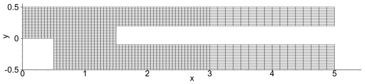
- [§2.3, Theorem 2.1, and §3 numerical experiments] Theorem 2.1 is stated in the limit delta -> 0, while all numerical experiments use a finite smoothing parameter: delta = 0.05 in §3.2 and delta = 0.01 in §3.3 and §3.4. As written, the proof does not cover the finite-delta scheme actually tested. This gap is readily repairable: from (6) and (46), B0 = 1/2 int_{partial Omega_o} |bar u|^2 (n·bar u) tanh((n·bar u)/(U0 delta)) dA, which is nonnegative for every delta > 0. Thus the monotonicity conclusion (26) can be proved for finite delta without taking delta to 0. The authors should make this repair and state Theorem 2.1 for the finite-delta regime used in the computations.
minor comments (4)
- [Equations (26), (46)] The notation with doubled norm bars, || ||nabla bar u|| ||^2, appears to be a LaTeX artifact; please use a single norm notation throughout.
- [§3.2, bifurcation channel] The text refers to the 'no-clip condition' on the walls; this should be the 'no-slip condition'.
- [§2.4, positivity of xi] The claim that xi > 0 unconditionally should be qualified: in the homogeneous case S1 = 0 and the numerator of (45) is (R^{n+1/2})^2, so xi = 0 if R^{n+1/2} = 0. If this exceptional case is possible, the authors should either rule it out or state the positivity claim for R^{n+1} only, which follows from (47).
- [Affiliation and references] There are minor typographical errors: 'Collge of Infomation Science' in the author affiliation and 'International Jurnal for Numerical Methods in Fluids' in reference [53].
Circularity Check
Theorem 2.1's R-decrease is an algebraic identity: ξ (Eq. 45) and R^{n+3/2} (Eq. 47) are defined so that (26) holds by construction; no bound on the physical energy E[u^{n+1}] follows.
-
self definitional
[Section 2.3-2.4, Theorem 2.1, Eq. (26), Eq. (45), Eq. (47)]
"Using equation (20b), we can compute ξ from (27) as follows, ξ = ((R^{n+1/2})^2 + S1∆t)/(E[¯u^{n+3/2}] + (A0 + B0 + S0)∆t). ... R^{n+1} is computed as follows, R^{n+3/2} = sqrt(ξE[¯u^{n+3/2}]), R^{n+1} = 2/3 R^{n+3/2} + 1/3 R^n."
Under the hypotheses of Theorem 2.1 (f = p0 = fb = w = 0), equations (28) give S0 = S1 = 0. Then (45) fixes ξ = (R^{n+1/2})^2 / (E[¯u^{n+3/2}] + (A0 + B0)∆t), and (47) fixes R^{n+3/2} = sqrt(ξ E[¯u^{n+3/2}]). Substituting these two definitions into (27) yields exactly (26): (R^{n+3/2})^2 - (R^{n+1/2})^2 = -ξ∆t(A0 + B0) ≤ 0. The stability inequality is therefore an identity produced by the formulas for ξ and R, not an independent estimate of the computed velocity. Moreover, R is not the physical discrete energy: the paper states that R^2(t) is 'an approximation of E(t), rather than E(t) itself,' and only ξ > 0 is proven, with no lower bound, so E[¯u] is not controlled when ξ tends to 0. The headline 'unconditionally energy-stable' rests on a quantity that is defined to decrease.
full rationale
The central stability theorem is self-definitional rather than an independent energy estimate. After solving the decoupled field equations for u1, u2, p1, p2, the scalar ξ is computed from equation (45) precisely so that equation (27) becomes the desired dissipation identity, and R^{n+3/2} is then defined from that same ξ in (47). Consequently Theorem 2.1's inequality is true by construction, exactly as in the pattern 'parameter fitted so that the predicted ratio is the fit.' The paper itself concedes the auxiliary-variable status: 'Note that R(t) is obtained by solving this coupled system of equations, not by using equation (11). So in such a sense R^2(t) is an approximation of E(t), rather than E(t) itself.' No lower bound on ξ is established, and the actual velocity is u^{n+1} = u1 + g(ξ)u2 while the dissipation in (26) is evaluated on ¯u^{n+1} = u1 + u2; thus boundedness of R^2 does not imply boundedness of the physical velocity energy. The numerical experiments are extensive and show stable behavior, but they do not repair the gap: the paper's unconditional stability claim reduces to the monotonicity of a scalar that the algorithm defines to be monotone. There is also self-citation of the gPAV source [54], but the derivation in this paper is self-contained once the auxiliary-variable framework is accepted, so no additional circularity score is assigned for that citation. The score is 6 because the central claim is partially circular: the auxiliary-energy inequality is enforced by construction, while the scheme still has independent algorithmic content (decoupled constant-matrix solves, positivity of ξ, and reproducible numerical results).
Assumptions & free parameters
free parameters (3)
- D0 =
1 (tests; varied 0.1 to 2.0)
- delta =
0.05 and 0.01 in tests
- C0 =
1 (tests; varied 1e-3 to 1e6)
assumptions (4)
- domain assumption The convective-like energy-stable open boundary condition (5) from Dong (2015) is stable at the PDE level.
- standard math The gPAV-reformulated system (14) and (17) is equivalent to the original Navier-Stokes system because R^2/E = 1 and g(R^2/E) = 1 at the continuum.
- domain assumption For sufficiently small delta, the boundary integral B0 in (46) is nonnegative.
- standard math BDF2 plus explicit second-order extrapolation for the convective term is second-order accurate.
invented entities (3)
-
Auxiliary variable R(t)
-
Scaling factor xi
-
g(chi) function
Cite this review
Pith. "Pith review of A gPAV-Based Unconditionally Energy-Stable Scheme for Incompressible Flows with Outflow/Open Boundaries." pith.science (2026). https://pith.science/paper/BKLTEWHO
@misc{pith2026190801852,
  author       = {Pith},
  title        = {Pith review of: A gPAV-Based Unconditionally Energy-Stable Scheme for Incompressible Flows with Outflow/Open Boundaries},
  year         = {2026},
  howpublished = {\url{https://pith.science/paper/BKLTEWHO}},
  note         = {Machine review of arXiv:1908.01852}
}
read the original abstract
We present an unconditionally energy-stable scheme for approximating the incompressible Navier-Stokes equations on domains with outflow/open boundaries. The scheme combines the generalized Positive Auxiliary Variable (gPAV) approach and a rotational velocity-correction type strategy, and the adoption of the auxiliary variable simplifies the numerical treatment for the open boundary conditions. The discrete energy stability of the proposed scheme has been proven, irrespective of the time step sizes. Within each time step the scheme entails the computation of two velocity fields and two pressure fields, by solving an individual de-coupled Helmholtz (including Poisson) type equation with a constant pre-computable coefficient matrix for each of these field variables. The auxiliary variable, being a scalar number, is given by a well-defined explicit formula within a time step, which ensures the positivity of its computed values. Extensive numerical experiments with several flows involving outflow/open boundaries in regimes where the backflow instability becomes severe have been presented to test the performance of the proposed method and to demonstrate its stability at large time step sizes.
Figures


Figures from the paper (15 more)







Reference graph
Works this paper leans on
-
[18]
S. Dong and J. Shen. An unconditionally stable rotational velocity-correction scheme for incompressible flows. Journal of Computational Physics , 229:7013–7029, 2010
work page 2010
-
[1]
M.O. Abu-Al-Saud, A. Riaz, and H.A. Tchelepi. Multiscale level-set method for accurate modeling of immiscible two-phase flow with deposited thin films on solid surfaces.Journal of Computational Physics, 333:297–320, 2017
work page 2017
-
[2]
Y. Bazilevs, J.R. Hohean, T.J.R. Hughes, R.D. Moser, and Y. Zhang. Patient-specific isogeometric fluid-structure interaction analysis of theracic aortic blood flow due to impantation of the jarvik 2000 left ventricular assist device. Comput. Methods Appl. Mech. Engrg. , 198:3534–3550, 2009
work page 2000
-
[3]
C. Bertoglio and A. Caiazzo. A tangential regularization method for backflow stabilization in hemody- namics. Journal of Computational Physics , 261:162–171, 2014
work page 2014
-
[4]
C. Bertoglio and A. Caiazzo. A stokes-residual backflow stabilization method applied to physiological flows. Journal of Computational Physics , 313:260–278, 2016
work page 2016
- [5]
-
[6]
C.-H. Bruneau and P. Fabrie. Effective downstream boundary conditions for incompressible Navier- Stokes equations. International Journal for Numerical Methods in Fluids , 19:693–705, 1994
work page 1994
-
[7]
C.-H. Bruneau and P. Fabrie. New efficient boundary conditions for incompressible navier-stokes equa- tions: a well-posedness result. Mathematical Modeling and Numerical Analysis , 30:815–840, 1996
work page 1996
Show all 57 references
-
[8]
H. Chen, S. Sun, and T. Zhang. Energy stability analysis of some fully discrete numerical schemes for incompressible navier-stokes equations on staggered grids. Journal of Scientific Computing , 75:427–456, 2018
2018
-
[9]
L. Chen, J. Shen, and C.J. Xu. A unstructured nodal spectral-element method for the navier-stokes equations. Communications in Computational Physics , 12:315–336, 2012
2012
-
[10]
A.J. Chorin. Numerical solution of the Navier-Stokes equations. Math. Comput., 22:745–762, 1968
1968
-
[11]
S. Dong. Evidence for internal structures of spiral turbulence. Physical Review E, 80:067301, 2009
2009
-
[12]
S. Dong. An efficient algorithm for incompressible N-phase flows. Journal of Computational Physics , 276:691–728, 2014
2014
-
[13]
S. Dong. An outflow boundary condition and algorithm for incompressible two-phase flows with phase field approach. Journal of Computational Physics , 266:47–73, 2014
2014
-
[14]
S. Dong. A convective-like energy-stable open boundary condition for simulations of incompressible flows. Journal of Computational Physics , 302:300–328, 2015
2015
-
[15]
S. Dong. Wall-bounded multiphase flows of N immiscible incompressible fluids: consistency and contact- angle boundary condition. Journal of Computational Physics , 338:21–67, 2017
2017
-
[16]
Dong, G.E
S. Dong, G.E. Karniadakis, and C. Chryssostomidis. A robust and accurate outflow boundary condition for incompressible flow simulations on severely-truncated unbounded domains.Journal of Computational Physics, 261:83–105, 2014
2014
-
[17]
Dong, G.E
S. Dong, G.E. Karniadakis, A. Ekmekci, and D. Rockwell. A combined direct numerical simulation- particle image velocimetry study of the turbulent near wake. J. Fluid Mech. , 569:185–207, 2006
2006
-
[19]
Dong and J
S. Dong and J. Shen. A time-stepping scheme involving constant coefficient matrices for phase field simulations of two-phase incompressible flows with large density ratios. Journal of Computational Physics, 231:5788–5804, 2012
2012
-
[20]
Dong and J
S. Dong and J. Shen. A pressure correction scheme for generalized form of energy-stable open boundary conditions for incompressible flows. Journal of Computational Physics , 291:254–278, 2015
2015
-
[21]
Dong and X
S. Dong and X. Wang. A rotational pressure-correction scheme for incompressible two-phase flows with open boundaries. PLOS One, 11(5):e0154565, 2016
2016
-
[22]
Ghaisas, D.A
N.S. Ghaisas, D.A. Shetty, and S.H. Frankel. Large eddy simulation of turbulent horizontal buoyant jets. Journal of Turbulence, 16:772–808, 2015
2015
-
[23]
Gravemeier, A
V. Gravemeier, A. Comerford, L. Yoshihara, M. Ismail, and W.A. Wall. A novel formulation for Neumann inflow boundary conditions in biomechanics. International Journal for Numeical Methods in Biomedical Engineering, 28:560–573, 2012
2012
-
[24]
P.M. Gresho. Incompressible fluid dynamics: some fundamental formulation issues. Annual Review of Fluid Mechanics, 23:413–453, 1991
1991
-
[25]
Guermond, P
J.L. Guermond, P. Minev, and J. Shen. Error analysis of pressure-correction schemes for the time- dependent stokes equations with open boundary conditions. SIAM J. Numer. Anal. , 43:239–258, 2005. 32
2005
-
[26]
Guermond, P
J.L. Guermond, P. Minev, and J. Shen. An overview of projection methods for incompressible flows. Comput. Methods Appl. Mech. Engrg. , 195:6011–6045, 2006
2006
-
[27]
Guermond and J
J.L. Guermond and J. Shen. A new class of truly consistent splitting schemes for incompressible flows. J. Comput. Phys. , 192:262–276, 2003
2003
-
[28]
Hyoungsu and G.E
B. Hyoungsu and G.E. Karniadakis. Subiteration leads to accuracy and stability enhancements of semi- implicit schemes for the navier-stokes equations. Journal of Computational Physics , 230:4384–4402, 2011
2011
-
[29]
Ismail, V
M. Ismail, V. Gravemeier, A. Comerford, and W.A. Wall. A stable approach for coupling multidi- mensional cardiovascular and pulmonary networks based on a novel pressure-flow rate or pressure-only neumann boundary condition formulation. International Journal for Numerical Method...
2014
-
[30]
Jiang, M
N. Jiang, M. Mohebujjaman, L.G. Rebholz, and C. Trenchea. An optimally accurate discrete regulariza- tion for second order timestepping methods for navier-stokes equations. Comput. Methods Appl. Mech. Engrg., 310:388–405, 2016
2016
-
[31]
Karniadakis, M
G.E. Karniadakis, M. Israeli, and S.A. Orszag. High-order splitting methods for the incompressible Navier-Stokes equations. J. Comput. Phys. , 97:414–443, 1991
1991
-
[32]
Karniadakis and S.J
G.E. Karniadakis and S.J. Sherwin. Spectral/hp element methods for computational fluid dynamics, 2nd edn. Oxford University Press, 2005
2005
-
[33]
Kim and P
J. Kim and P. Moin. Application of a fractional-step method to incompressible Navier-Stokes equations. J. Comput. Phys. , 59:308–323, 1985
1985
-
[34]
Kravchenko and P
A.G. Kravchenko and P. Moin. Numerical studies of flow over a circular cylinder at ReD = 3900. Physics of Fluids, 12:403–417, 2000
2000
-
[35]
Labovsky, W.J
A. Labovsky, W.J. Layton, C.C. Manica, M. Neda, and L.G. Rebholz. The stabilized extrapolated trape- zoidal finite-element method for the Navier-Stokes equations. Comput. Methods Appl. Mech. Engrg. , 198:958–974, 2009
2009
-
[36]
M.S. Lee, A. Riaz, and V. Aute. Direct numerical simulation of incompressible multiphase flow with phase change. Journal of Computational Physics , 344:381–418, 2017
2017
-
[37]
L. Lin, Z. Yang, and S. Dong. Numerical approximation of incompressible Navier-Stokes equations based on an auxiliary energy variable. Journal of Computational Physics , 388:1–22, 2019
2019
-
[38]
J.-G. Liu, J. Liu, and R.L. Pego. Stability and convergence of efficient Navier-Stokes solvers via a commutator estimate. Comm. Pure Appl. Math. , LX:1443–1487, 2007
2007
-
[39]
Moghadam, Y
M.E. Moghadam, Y. Bazilevs, T.-Y. Hsia, I.E. Vignon-Clementel, and A.L. Marsden. A comparison of outlet boundary treatments for prevention of backflow divergence with relevance to blood flow simula- tions. Comput. Mech., 48:277–291, 2011
2011
-
[40]
N. Ni, Z. Yang, and S. Dong. Energy-stable boundary conditions based on a quadratic form: Applica- tions to outflow/open-boundary problems in incompressible flows. Journal of Computational Physics , 391:179–215, 2019
2019
-
[41]
Porpora, P
A. Porpora, P. Zunino, C. Vergara, and M. Piccinelli. Numerical treatment of boundary conditions to replace branches in hemodynamics. International Journal of Numerical Methods in Biomedical Engi- neering, 28:1165–1183, 2012
2012
-
[42]
A. Poux, S. Glockner, and M. Azaiez. Improvements on open and traction boundary conditions for navier-stokes time-splitting methods. Journal of Computational Physics , 230:4011–4027, 2011. 33
2011
-
[43]
Sanderse
B. Sanderse. Energy-conserving runge-kutta methods for the incompressible navier-stokes equations. J. Comput. Phys., 233:100–131, 2013
2013
-
[44]
Serson, J.R
D. Serson, J.R. Meneghini, and S.J. Sherwin. Velocity-correction schemes for the incompressible navier- stokes equations in general coordinate systems. Journal of Computational Physics , 316:243–254, 2016
2016
-
[45]
J. Shen. On error estimate of projection methods for Navier-Stokes equations: first-order schemes. SIAM J. Numer. Anal. , 29:57–77, 1992
1992
-
[46]
J. Shen, J. Xu, and J. Yang. The scalar auxiliary variable (sav) approach for gradient flows. Journal of Computational Physics, 353:407–416, 2018
2018
-
[47]
Sherwin and G.E
S.J. Sherwin and G.E. Karniadakis. A triangular spectral element method: applications to the incom- pressible navier-stokes equations. Comput. Meth. Appl. Mech. Engrg. , 123:189–229, 1995
1995
-
[48]
Simo and F
J.C. Simo and F. Armero. Unconditional stability and long-term behavior of transient algorithms for the incompressible Navier-Stokes and Euler equations. Comput. Methods Appl. Mech. Engrg. , 111:111–154, 1994
1994
-
[49]
R. Temam. Sur l’approximation de la solution des equations de Navier-Stokes par la methods des pas fractionnaires ii. Arch. Ration. Mech. Anal., 33:377–385, 1969
1969
-
[50]
Varghese, S.H
S.S. Varghese, S.H. Frankel, and P.F. Fischer. Direct numerical simulation of stenotic flows. Part 1. steday flow. Journal of Fluid Mechanics , 582:253–280, 2007
2007
-
[51]
Verstappen and A.E.P
R.W.C.P. Verstappen and A.E.P. Veldman. Symmetry-preserving discretization of turbulent flow. Jour- nal of Computational Physics , 187:343–368, 2003
2003
-
[52]
Williamson
C.H.K. Williamson. Vortex dynamics in a cylinder wake. Annual Review of Fluid Dynamics, 28:477–539, 1996
1996
-
[53]
Xu and R
C.J. Xu and R. Pasquetti. On the efficiency of semi-implicit and semi-lagrangeian spectral methods for the calculation of incompressible flows. International Jurnal for Numerical Methods in Fluids , 35:319– 340, 2001
2001
-
[54]
Yang and S
Z. Yang and S. Dong. A roadmap for discretely energy-stable schemes for dissipative systems based on a generalized auxiliary variable with guaranteed positivity. arXiv:1904.00141
1904 arXiv
-
[55]
Yang and S
Z. Yang and S. Dong. An unconditionally energy-stable scheme based on an implicit auxiliary en- ergy variable for incompressible two-phase flows with different densities involving only precomputable coefficient matrices. Journal of Computational Physics , 393:229–257, 2019
2019
-
[56]
Z. Yang, L. Lin, and S. Dong. A family of second-order energy-stable schemes for Cahn-Hilliard type equations. Journal of Computational Physics , 383:24–54, 2019
2019
-
[57]
Zheng and S
X. Zheng and S. Dong. An eigen-based high-order expansion basis for structured spectral elements. Journal of Computational Physics , 230:8573–8602, 2011. 34
2011
Reviewed August 14, 2026 · model on record in the stance chip above.
Discussion (0). Continue with ORCID to comment.