Finite-Horizon Optimal Control of Boolean Control Networks: A Unified Graph-Theoretical Approach

Changkai Sun; Cheng Xiang; Kairong Qin; Shuhua Gao; Tong Heng Lee

REVIEW 3 major objections 6 minor 36 references

Finite-Horizon Optimal Control of Boolean Control Networks: A Unified Graph-Theoretical Approach

T0 review · 3 major / 6 minor · reviewed 2026-08-14 · deepseek-v4-flash

Challenge this review Re-run · record.json Download PDF Read on arXiv ↗ Review JSON

Pith's one-line read The paper proves that two general finite-horizon optimal control problems for Boolean control networks—fixed horizon and fixed destination, both allowing time-variant costs—are exactly shortest-path problems in tailored state-transition…

desk verdict A real unification of BCN optimal control into shortest path problems, with an honest but load-bearing monotonicity assumption and a few missing details worth fixing. read the letter →

arxiv 1908.02019 v2 pith:RNB6JIWM submitted 2019-08-06 math.OC

Shuhua Gao , Changkai Sun , Cheng Xiang , Kairong Qin , Tong Heng Lee This is my paper · ORCID

classification math.OC MSC 93C5505C8590C35

keywords Booleancontrolnetworksfinite-horizonoptimalshortestpathproblemstatetransitiongraphtime-expandeddynamicprogrammingDijkstra'salgorithmtime-variantcosts

verification ladder T0 review T1 audit T2 compute T3 formal

The pith

A machine-rendered reading of the paper's core claim, the machinery that carries it, and where it could break.

The reading

Boolean control networks are deterministic networks of on/off variables, typically gene states, whose evolution is driven by binary inputs; choosing an input sequence to minimize a cost over a finite planning window is a core task for designing interventions. The paper claims that two very general forms of this task, one with a fixed number of steps (Problem 1) and one with an unknown but finite number of steps ending in a target set (Problem 2), can be reformulated exactly as shortest-path problems on specially constructed graphs, even when costs vary with time and when states and inputs are constrained. This unification means that previously scattered special cases—minimum-energy control, minimum-time control, Mayer-type problems, time-discounted costs, and others—are all captured by one graph-theoretic machinery, and the paper derives worst-case running times of $O(TMN)$, $O(MN+N\log N)$, and $O(N^2(M+2\log N))$, where $N$ is the number of states and $M$ is the number of control inputs. A sympathetic reader would care because the paper also claims the first solution to fixed-destination optimal control with time-variant costs, and on the Ara-operon benchmark the graph methods are several orders of magnitude faster than algebraic matrix-based methods.

What carries the argument

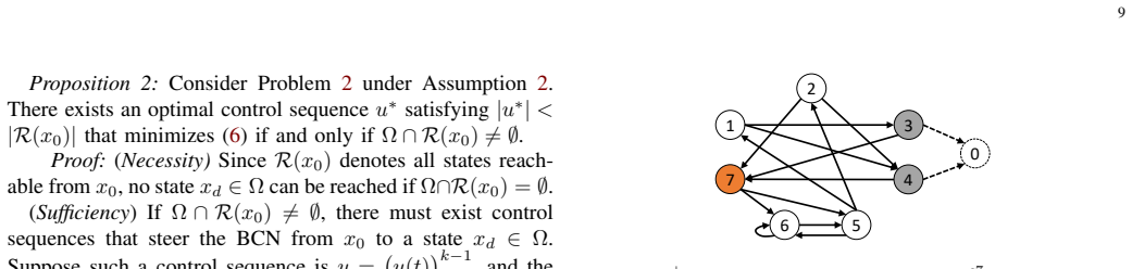
The load-bearing object is the state transition graph (STG) of the Boolean control network: vertices are the states reachable from a given initial state, and a directed edge exists for each one-step transition; edge weights are set to the minimum stage cost among the controls that realize the transition. Around this object the paper builds three variants: the TET-STG (layered by time, for fixed horizons), the STG+ (a static graph with a pseudo-state for terminal costs, for time-invariant fixed-destination problems), and the TED-STG (time-expanded layers up to $|R(x_0)|-1$, with pseudo-state edges from every destination occurrence, for time-variant fixed-destination problems). The pseudo-state $\delta^0_N$ is the device that converts a terminal cost into an edge weight. The reduction is carried by the fact that any feasible control sequence maps to a path whose weight is at most the control cost, with equality when each transition uses the cheapest admissible control; combined with finiteness of the candidate set, this turns planning into an unconstrained shortest-path computation.

What would settle it

For a small Boolean control network with $|R(x_0)|=3$, choose time-variant costs that satisfy Assumption 2—for example $g(t)=1$ for $t<3$ and $g(t)=2$ afterwards, with zero terminal cost—and compare Algorithm S1's returned plan to exhaustive enumeration of all control sequences of lengths 1 through 5 under the same state and control constraints. If any enumerated sequence yields strictly smaller total cost, Theorem 4's reduction to a shortest path in the TED-STG is false; otherwise the claim survives this check.

Watch

Extended reading notes

Core claim

The paper's central claim is a reduction. The fixed-time problem (Problem 1) is equivalent to a shortest-path problem in the time-expanded fixed-time state transition graph (TET-STG), which places one copy of each reachable state at each time step and adds a pseudo-state to absorb the terminal cost; the optimal cost is the weight of a shortest path from the initial state at time 0 to that pseudo-state, and the optimal control sequence is read off from the minimizing controls along the path. For the fixed-destination problem with time-invariant costs, the extended state transition graph (STG+) adds a terminal pseudo-state to the ordinary state graph, and the problem becomes a standard single-pair shortest-path problem solved by Dijkstra's algorithm (Algorithm 3). For time-variant costs in the fixed-destination problem, the time-expanded fixed-destination state transition graph (TED-STG) stacks the reachable states over all times up to $|R(x_0)|-1$ and connects every occurrence of a destination state to the pseudo-state, so the problem again becomes a single-pair shortest-path problem (Algorithm S1). Equality between the optimal control cost and the shortest-path weight is shown by pairing each control sequence with a path whose weight never exceeds the control cost, and by noting that the optimal one-step control on each transition attains equality.

Load-bearing premise

The paper's fixed-destination results require that per-step costs never be negative and that both per-step and terminal costs never decrease as time goes on; if later steps could become cheaper, looping around a cycle could make total cost arbitrarily small and no finite optimal plan would exist.

Editorial extensions

If this is right

The same graph pipeline solves every special case listed in the literature—minimum-energy, minimum-time, Mayer-type, Lagrange-type, and time-discounted problems—without needing a new method for each case.
Fixed-destination optimal control with time-variant costs, previously unsolved, is solvable in $O(N^2(M+2\log N))$ worst-case time, compared with the $O(MN^3)$ cost of checking every horizon length with a fixed-time solver.
Because the graphs are built only from the reachable set $R(x_0)$, the algorithms exploit networks whose reachable part is small; on the Ara-operon example the reachable set has 108 states out of 512.
For fixed-horizon problems, the equivalence holds even with negative edge weights, since the horizon is fixed and cycles cannot be exploited; only bounded-below costs are required.

Reading between the lines

Editorial extensions of the paper, not claims the author makes directly.

The paper does not treat stochastic networks, but the same time-expanded construction would apply to probabilistic Boolean networks if edge weights were replaced by expected stage costs, although the shortest-path equivalence would then need a careful treatment of probabilities.
A natural stress test of the framework is to run Algorithm S1 on networks where $|R(x_0)|$ is close to $N$; the complexity advantage over algebraic methods comes mostly from sparse reachability, so dense networks would erase much of the reported speed-up.
The monotonicity assumption in Assumption 2 is what makes the finite bound $|u^*|<|R(x_0)|$ hold; the paper's fixed-destination results are best read as showing that time-variant costs are tractable precisely when waiting never makes travel cheaper.

Share X Bluesky LinkedIn Reddit HN

Signed reviews

No signed human review yet.

Editorial analysis

A structured set of objections, weighed in public.

Desk editor's note, referee report, and a circularity audit.

Desk Editor's Note

read the letter

Read arXiv:1908.02019. The core contribution holds up: Problem 1 (fixed horizon) and Problem 2 (fixed destination) for Boolean control networks are reduced to shortest path problems in STG-based graphs, including time-variant costs and constraints. That is genuinely new compared with [14] and [23], which only handle time-invariant special cases. The TET-STG plus DP algorithm is standard but clean; the TED-STG construction for time-variant fixed-destination costs is the most original piece. The worst-case bounds O(TMN), O(MN + N log N), and O(N^2(M + 2 log N)) check out, and the paper ships Python code, which I respect.

The mathematical architecture is sound. Theorems 1 through 4 are straightforward proofs of the reductions, and Proposition 2's cycle-elimination argument is valid under Assumption 2. I do not see fitted parameters, circular reasoning, or overclaimed credit: the authors explicitly acknowledge the earlier graph-based work of [14] and [23].

The big caveat is Assumption 2, and it is load-bearing. For fixed-destination problems, the paper requires h bounded below and g nonnegative, with both nondecreasing in time. The stress-test example is correct: with a zero-cost self-loop and a time-decreasing edge cost to the destination, the optimal sequence can wait many steps before taking the cheap edge, so the bound K < |R(x0)| and hence the finite TED-STG construction fail. The paper states Assumption 2 explicitly, which is to its credit, but the abstract and contribution list say "time-variant costs" without the monotonicity qualifier. That overstates the scope. The fix is easy in presentation: keep the assumption and say plainly in the abstract that time-varying costs must be nondecreasing, or extend the theory, which is not obvious.

Minor issues: Lemma 5's proof is omitted, though it is nearly identical to Lemma 3, so this is minor. The benchmark timing table is missing from the supplied text (Table ??), and the running times have no error bars or iteration counts. The Ara operon results are illustrative, not load-bearing, and the missing table should be restored before publication.

Who is this for? Anyone working on BCN optimal control who wants to replace STP matrix algebra with graph algorithms. It deserves a serious referee and, after a revision that fixes the scope wording and supplies the missing benchmark details, it should be accepted. I would cite it and would bring it to a reading group on control of Boolean networks.

Referee Report

3 major / 6 minor

Summary. The paper proposes a unified graph-theoretic framework for finite-horizon optimal control (FHOC) of Boolean control networks. Two general problems are formulated: Problem 1 with a fixed horizon T and Problem 2 with an unspecified finite horizon to a destination set, both allowing time-variant costs and state/control constraints. The authors construct weighted state transition graphs and time-expanded variants (TET-STG, STG+, TED-STG), prove in Theorems 1-4 that the two FHOC problems are equivalent to shortest-path problems in these graphs, and develop Algorithm 2 (DP over the TET-STG), Algorithm 3 (modified Dijkstra over STG+), and Algorithm S1 (modified Dijkstra over TED-STG). Worst-case complexities O(TMN), O(MN + N log N), and O(N^2(M + 2 log N)) are claimed. The paper reports an application to the Ara operon network of E. coli and claims substantial running-time improvements over existing algebraic methods.

Significance. If the results hold, the paper gives a clean and useful unification: rather than developing separate algebraic algorithms for each FHOC variant, all considered problems are reduced to shortest-path computations on explicitly constructed graphs. The reduction proofs for Theorems 1-4 are carefully structured, the complexity analyses of the three algorithms check out, and the worked examples are simple enough to verify by inspection. A particular strength is that the approach genuinely handles time-variant stage and terminal costs for Problem 1, and time-nondecreasing time-variant costs for Problem 2, which goes beyond most prior work. The benchmark on the Ara operon network is potentially valuable, although the reported timing data are missing from the manuscript. The central theoretical contribution is sound under the stated assumptions, but the scope of the time-variant claim for Problem 2 needs to be qualified.

major comments (3)

[Section VI.A, Assumption 2 and Definition 7/Theorem 4] The monotonicity condition (iii) in Assumption 2 is load-bearing for the fixed-destination results, and the unqualified claim of solving Problem 2 with time-variant costs is too strong without it. Proposition 2's cycle-elimination argument in Eq. (21) uses h(xd,k) >= h(xd,k-r) and g(x(t),u(t),t) >= g(x(t),u(t),t-r); if g can decrease over time, removing a cycle can increase cost, so the bound |u*| < |R(x0)| that fixes the number of layers in Definition 7 is invalid. A concrete two-state example: let R(x0)={x0,xd}, place a zero-cost self-loop on x0, set the edge x0->xd to cost max(10-t,0), and set h=0, Omega={xd}. Every optimal sequence waits at least 10 steps and then moves, with cost 0 and K>=11, but the TED-STG with Z=2 contains only the t=0 transition and Dijkstra's algorithm on it returns cost 10. Thus Algorithm S1 and Theorem 4 solve Problem 2 with time-variant costs only under time-nondecreasing costs; the abstract, the contribution list, and the Table I row for Algorithm S1 should state this restriction explicitly.
[Section VIII.A/B, 'Table ??'] The benchmark timing measurements are not actually reported. The text refers to 'Table ??' twice, once in Task 1 and once in Task 2, but no such table appears in the manuscript. Since the abstract claims that the approach 'can dramatically reduce the running time' and Remark 13 repeats this claim, the missing table is load-bearing for the empirical part of the paper. The authors should supply the timing table with the measured running times of the compared methods, or explicitly qualify the empirical claims as unsupported pending additional experiments.
[Section VI.C, Lemma 5] The proof of Lemma 5 is omitted with the statement that it can be proved 'in almost the same way as Lemma 3'. Because Theorem 4 relies on Lemma 5 to relate feasible control sequences to paths in the TED-STG, the proof should be included or, at minimum, the t-shift argument that handles the time-dependent terminal cost h(x(K),K) should be spelled out. This is a short argument, but an omitted load-bearing lemma is a gap in the published proof chain as written.

minor comments (6)

[Algorithm S1] The pseudo-state is labeled delta_0_N,N in the implementation, while Definition 7 gives the pseudo-state no time index; please clarify this implementation label to avoid confusion between N (number of BCN states) and Z (reachable-set size).
[Section V.C] The phrase 'Combing Theorem 1 and 2' should read 'Combining Theorem 1 and 2'.
[Example 3] The sentence 'enumerating all paths from delta_1_4,0 to delta_0_4,5' appears to have state subscripts 4 instead of 8; the TET-STG in Fig. 2 is built from states of the form delta_i_8.
[Section IV] There are minor typos: 'bread-first search' should be 'breadth-first search', and 'intial state' should be 'initial state'.
[Section VIII.A] In the bullet list of Task 1 results, 'the complete state state has 512 states' has a duplicated word; it should read 'the complete state space has 512 states'.
[Algorithm 3, line 18] The notation 'uij (15)' refers to a formula defined for the time-variant TET-STG; in the time-invariant setting of Definition 6 the control uij has no time superscript, so the reference should be adjusted for consistency.

Circularity Check

0 steps flagged · score 0.0 of 10

No circularity found: the shortest-path reductions are proved equivalences from explicit problem data, not renamed inputs.

full rationale

The paper's central claim is that the two FHOC problems can be reduced to shortest-path problems in explicitly constructed time-expanded graphs. The reduction is a direct mathematical equivalence: edge weights in the TET-STG are defined by Eq. (14) as the minimal stage cost for each transition plus the terminal cost, and Lemma 3 / Theorem 1 prove that for every feasible control sequence the objective JT(u) equals the weight of the corresponding path, and conversely every path yields a feasible control sequence with the same cost. No parameter is fitted to data and then renamed a prediction; the cost matrices in the examples are arbitrary illustrations, and any correct algorithm would return the same optimum. The benchmark uses standard literature instances and compares only running time, so there is no post hoc selection that could force the claimed efficiencies. There are no load-bearing self-citations: prior-work references are to independent authors, and the graph constructions are defined in this paper rather than imported from cited work. The only notable scope restriction is Assumption 2 in Section VI.A, which imposes nonnegative and time-nondecreasing costs; the paper states this assumption explicitly and uses it to prove the cycle-elimination bound |u*| < |R(x0)| in Proposition 2 and to justify the TED-STG construction in Theorem 4. That is a genuine modeling limitation on the generality of Problem 2 with time-variant costs, but it is not circular: the paper does not assume the result it proves. Overall, the derivation is self-contained and no circular step reduces the claimed results to their own inputs.

Assumptions & free parameters 0 free parameters · 5 assumptions · 2 invented entities

The central argument relies on the standard STP/ASSR representation of BCNs and on classical shortest path algorithms, plus two stated cost assumptions, Assumptions 1 and 2. No free parameters are fitted. The pseudo-state and time-expanded copies are graph bookkeeping devices, not empirical postulates.

assumptions (5)

standard math The STP ASSR representation x(t+1) = L u(t) x(t) exactly captures the dynamics of any BCN (Lemma 1).
Invoked throughout Sections IV through VIII; the equivalence between Boolean functions and logical matrices is a known result from references [6] and [7].
domain assumption Assumption 1: stage cost g and terminal cost h_T in Problem 1 are bounded below.
Stated in Section V.A; guarantees the finite candidate set has a minimum. Not true for arbitrary cost functions, so it restricts the claimed generality.
domain assumption Assumption 2: h is bounded below, g is nonnegative, and both are nondecreasing in time t.
Stated in Section VI.A; load-bearing for Proposition 2 and Theorem 4 because cycle removal relies on nonnegative and time-nondecreasing costs.
standard math Dijkstra's algorithm and the Bellman recursion correctly solve shortest path problems on graphs with nonnegative weights and no negative cycles.
Used in Theorems 2 through 4 and Algorithms 2, 3, and S1; standard results from reference [33], not proved in the paper.
standard math Any trajectory with at least |R(x0)|+1 states contains a repeated state, so a cycle can be removed without disconnecting the trajectory.
Pigeonhole principle used in Proposition 2 and Theorem 4 to bound the optimal horizon length by |R(x0)|-1.

invented entities (2)

Pseudo-state delta_0^N added to TET-STG, STG+, and TED-STG.
purpose: A single sink vertex that absorbs terminal costs h via incoming edges, so every feasible control trajectory maps to a path to one vertex.
It is an internal graph device, not an empirical object. It only re-encodes terminal costs and does not add predictive content.
Time-expanded copies of states, delta_i,t, in TET-STG and TED-STG.
purpose: Represent the same Boolean state at different time steps so that time-dependent edge weights become static per layer.
Standard space-time network construction from reference [34]; a bookkeeping device rather than a new physical entity.

how reviews work

0 comments

Cite this review

Pith. "Pith review of Finite-Horizon Optimal Control of Boolean Control Networks: A Unified Graph-Theoretical Approach." pith.science (2026). https://pith.science/paper/RNB6JIWM

@misc{pith2026190802019,
  author       = {Pith},
  title        = {Pith review of: Finite-Horizon Optimal Control of Boolean Control Networks: A Unified Graph-Theoretical Approach},
  year         = {2026},
  howpublished = {\url{https://pith.science/paper/RNB6JIWM}},
  note         = {Machine review of arXiv:1908.02019}
}

abstract

This paper investigates the finite-horizon optimal control (FHOC) problem of Boolean control networks (BCNs) from a graph theory perspective. We first formulate two general problems to unify various special cases studied in the literature: (i) the horizon length is $\textit{a priori}$ fixed; (ii) the horizon length is unspecified but finite for given destination states. Notably, both problems can incorporate time-variant costs, which are rarely considered in existing work, and a variety of constraints. The existence of an optimal control sequence is analyzed under mild assumptions. Motivated by BCNs' finite state space and control space, we approach the two general problems in an intuitive and efficient way under a graph-theoretical framework. A weighted state transition graph and its time-expanded variants are developed, and the equivalence between the FHOC problem and the shortest path problem in specific graphs is established rigorously. Two custom algorithms are developed to find the shortest path and construct the optimal control sequence with lower time complexity, though technically a classical shortest-path algorithm in graph theory is sufficient for all problems. Compared with existing algebraic methods, our graph-theoretical approach can achieve state-of-the-art time efficiency while targeting the most general problems. Furthermore, our approach is the first one capable of solving Problem (ii) with time-variant costs. Finally, the Ara operon genetic network in $\textit{E. coli}$ is used as a benchmark example to validate the effectiveness of our approach, and the results of two tasks show that our approach can dramatically reduce the running time.

Figures

Figures reproduced from arXiv: 1908.02019 by the authors.

**Figure 1.** STG of the BCN (12) in Example 1. Each circle labeled i represents a state δ i 8 , and the arrows denote state transitions. A. Existence of Optimal Solutions As we will discuss next, the stage costs and the terminal costs in (5) are mapped to edge weights of a graph to reduce Problem 1 to an SP problem. It is known that the SP problem is well defined only if the graph contains no negative-weight cycles [33]. Nonethe… view at source ↗

**Figure 2.** TET-STG in Example 2 with the initial state x0 = δ 1 8 (the orange circle). A circle labeled i at time t denotes a vertex δ i 8,t. We highlight the terminal states in Ω by gray circles and the pseudo-state δ 0 8 by a dashed circle and dashed edges. The annotation of each edge (k, w) means that this transition is achieved with control δ k 4 at a cost of w (i.e., the edge’s weight). Note that the dashed edges going in… view at source ↗

**Figure 3.** STG+in Example 4 with the initial state x0 = δ 7 8 (in orange) and two destination states {δ 3 8 , δ4 8 } (in gray). The weight and the control associated with each edge are not shown here for clarity. Note that the dashed edges going into the pseudo-state δ 0 8 need no control. 2) Add into G the pseudo-state δ 0 N and its incoming edges, V ← V ∪ {δ 0 N }, E ← E ∪ E 0 where E0 = {(δ i N , δ0 N )|δ i N ∈ V ∩ Ω} with … view at source ↗

Figures from the paper (2 more)

**Figure 4.** Figure 4: TED-STG in Example 6 with an initial state x0 = δ 1 8 and a destination state δ 6 8 . The weight and the control associated with each edge are not shown here for clarity. Note that the pseudo-state δ 0 8 has no fixed timestamp. and J(u) = w(p) holds if δ kt M = u itit+…

**Figure 5.** Figure 5: The state transition graph of the Ara operon network with the initial [PITH_FULL_IMAGE:figures/full_fig_p013_5.png]

Discussion (0). Continue with ORCID to comment.

Reference graph

Works this paper leans on

36 extracted references · 35 canonical work pages

[14]

Minimum energy control and optimal-satisfactory control of boolean control network,

F. Li and X. Lu, “Minimum energy control and optimal-satisfactory control of boolean control network,” Physics Letters A, vol. 377, no. 43, pp. 3112–3118, 2013

work page 2013
[23]

Optimal control problem of boolean control networks: A graph-theoretical approach,

X. Cui, J.-E. Feng, and S. Wang, “Optimal control problem of boolean control networks: A graph-theoretical approach,” in 2018 Chinese Con- trol And Decision Conference (CCDC) . IEEE, 2018, pp. 4511–4516

work page 2018
[1]

Metabolic stability and epigenesis in randomly con- structed genetic nets,

S. A. Kauffman, “Metabolic stability and epigenesis in randomly con- structed genetic nets,” Journal of theoretical biology , vol. 22, no. 3, pp. 437–467, 1969

work page 1969
[2]

Boolean modeling of biological regulatory networks: a methodology tutorial,

A. Saadatpour and R. Albert, “Boolean modeling of biological regulatory networks: a methodology tutorial,” Methods, vol. 62, no. 1, pp. 3–12, 2013

work page 2013
[3]

External control in markovian genetic regulatory networks,

A. Datta, A. Choudhary, M. L. Bittner, and E. R. Dougherty, “External control in markovian genetic regulatory networks,” Machine learning , vol. 52, no. 1-2, pp. 169–191, 2003

work page 2003
[4]

Boolean network representation of contagion dynamics during a ﬁnancial crisis,

M. A. L. Caetano and T. Yoneyama, “Boolean network representation of contagion dynamics during a ﬁnancial crisis,” Physica A: Statistical Mechanics and its Applications , vol. 417, pp. 1–6, 2015

work page 2015
[5]

Controllability and observability of boolean control networks,

D. Cheng and H. Qi, “Controllability and observability of boolean control networks,” Automatica, vol. 45, no. 7, pp. 1659–1667, 2009

work page 2009
[6]

A linear representation of dynamics of boolean networks,

D. Cheng and H. Qi, “A linear representation of dynamics of boolean networks,” IEEE Transactions on Automatic Control , vol. 55, no. 10, pp. 2251–2258, 2010

work page 2010

Show all 36 references

[7]

Input-state incidence matrix of boolean control networks and its applications,

Y . Zhao, H. Qi, and D. Cheng, “Input-state incidence matrix of boolean control networks and its applications,” Systems & Control Letters , vol. 59, no. 12, pp. 767–774, 2010

2010
[8]

Observability of boolean networks: A graph-theoretic approach,

D. Laschov, M. Margaliot, and G. Even, “Observability of boolean networks: A graph-theoretic approach,” Automatica, vol. 49, no. 8, pp. 2351–2362, 2013

2013
[9]

On algorithms for state feedback stabilization of boolean control networks,

J. Liang, H. Chen, and Y . Liu, “On algorithms for state feedback stabilization of boolean control networks,” Automatica, vol. 84, pp. 10– 16, 2017

2017
[10]

The robustness of outputs with respect to disturbances for boolean control networks,

B. Li, Y . Liu, J. Lou, J. Lu, and J. Cao, “The robustness of outputs with respect to disturbances for boolean control networks,” IEEE transactions on neural networks and learning systems , 2019

2019
[11]

Control of large-scale boolean networks via network aggregation,

Y . Zhao, B. K. Ghosh, and D. Cheng, “Control of large-scale boolean networks via network aggregation,” IEEE transactions on neural net- works and learning systems , vol. 27, no. 7, pp. 1527–1536, 2015

2015
[12]

A maximum principle for single-input boolean control networks,

D. Laschov and M. Margaliot, “A maximum principle for single-input boolean control networks,” IEEE Transactions on Automatic Control , vol. 56, no. 4, pp. 913–917, 2010

2010
[13]

A pontryagin maximum principle for multi-input boolean control networks,

D. Laschov and M. Margaliot, “A pontryagin maximum principle for multi-input boolean control networks,” Recent advances in dynamics and control of neural networks , 2013

2013
[15]

Minimum-time control of boolean networks,

D. Laschov and M. Margaliot, “Minimum-time control of boolean networks,” SIAM Journal on Control and Optimization , vol. 51, no. 4, pp. 2869–2892, 2013

2013
[16]

Optimal control of boolean control networks,

E. Fornasini and M. E. Valcher, “Optimal control of boolean control networks,” IEEE Transactions on Automatic Control , vol. 59, no. 5, pp. 1258–1270, 2013

2013
[17]

On the optimal control of boolean control networks,

Q. Zhu, Y . Liu, J. Lu, and J. Cao, “On the optimal control of boolean control networks,” SIAM Journal on Control and Optimization , vol. 56, no. 2, pp. 1321–1341, 2018

2018
[18]

Receding horizon based feedback optimization for mix-valued logical networks,

D. Cheng, Y . Zhao, and T. Xu, “Receding horizon based feedback optimization for mix-valued logical networks,” IEEE Transactions on Automatic Control, vol. 60, no. 12, pp. 3362–3366, 2015

2015
[19]

Optimal control of logical control networks,

Y . Zhao, Z. Li, and D. Cheng, “Optimal control of logical control networks,” IEEE Transactions on Automatic Control , vol. 56, no. 8, pp. 1766–1776, 2011

2011
[20]

A ﬂoyd-like algorithm for optimization of mix-valued logical control networks,

Y . Zhao, “A ﬂoyd-like algorithm for optimization of mix-valued logical control networks,” in Proceedings of the 30th Chinese Control Confer- ence. IEEE, 2011, pp. 1972–1977

2011
[21]

Optimal control of ﬁnite-valued networks,

D. Cheng, Y . Zhao, and J.-B. Liu, “Optimal control of ﬁnite-valued networks,” Asian Journal of Control , vol. 16, no. 4, pp. 1179–1190, 2014

2014
[22]

Optimal control of boolean control networks with average cost: A policy iteration approach,

Y . Wu, X.-M. Sun, X. Zhao, and T. Shen, “Optimal control of boolean control networks with average cost: A policy iteration approach,” Auto- matica, vol. 100, pp. 378–387, 2019

2019
[24]

Finite horizon tracking control of boolean control networks,

Z. Zhang, T. Leifeld, and P. Zhang, “Finite horizon tracking control of boolean control networks,” IEEE Transactions on Automatic Control , vol. 63, no. 6, pp. 1798–1805, 2017

2017
[25]

Optimal constrained stationary intervention in gene regulatory net- works,

B. Faryabi, G. Vahedi, J.-F. Chamberland, A. Datta, and E. R. Dougherty, “Optimal constrained stationary intervention in gene regulatory net- works,” EURASIP Journal on Bioinformatics and Systems Biology , vol. 2008, no. 1, p. 620767, 2008

2008
[26]

Control of boolean networks: Hardness results and algorithms for tree structured networks,

T. Akutsu, M. Hayashida, W.-K. Ching, and M. K. Ng, “Control of boolean networks: Hardness results and algorithms for tree structured networks,” Journal of theoretical biology , vol. 244, no. 4, pp. 670–679, 2007

2007
[27]

An improved criterion for controllability of boolean control networks,

J. Liang, H. Chen, and J. Lam, “An improved criterion for controllability of boolean control networks,” IEEE Transactions on Automatic Control, vol. 62, no. 11, pp. 6012–6018, 2017

2017
[28]

Further results on the controllability of boolean control networks,

Q. Zhu, Y . Liu, J. Lu, and J. Cao, “Further results on the controllability of boolean control networks,” IEEE Transactions on Automatic Control, vol. 64, no. 1, pp. 440–442, 2018

2018
[29]

Optimal inﬁnite-horizon con- trol for probabilistic boolean networks,

R. Pal, A. Datta, and E. R. Dougherty, “Optimal inﬁnite-horizon con- trol for probabilistic boolean networks,” IEEE Transactions on Signal Processing, vol. 54, no. 6, pp. 2375–2387, 2006

2006
[30]

Discovery of a kernel for con- trolling biomolecular regulatory networks,

J. Kim, S.-M. Park, and K.-H. Cho, “Discovery of a kernel for con- trolling biomolecular regulatory networks,” Scientiﬁc reports, vol. 3, p. 2223, 2013

2013
[31]

The discrete linear time invariant time-optimal control probleman overview,

J. O’Reilly, “The discrete linear time invariant time-optimal control probleman overview,” Automatica, vol. 17, no. 2, pp. 363–370, 1981

1981
[32]

A minimum-time control for boolean control networks with impulsive disturbances,

H. Chen, B. Wu, and J. Lu, “A minimum-time control for boolean control networks with impulsive disturbances,”Applied Mathematics and Computation, vol. 273, pp. 477–483, 2016

2016
[33]

T. H. Cormen, C. E. Leiserson, R. L. Rivest, and C. Stein, Introduction to Algorithms, 3rd ed. The MIT Press, 2009

2009
[34]

Shortest path algorithms in trans- portation models: classical and innovative aspects,

S. Pallottino and M. G. Scutella, “Shortest path algorithms in trans- portation models: classical and innovative aspects,” in Equilibrium and advanced transportation modelling . Springer, 1998, pp. 245–281

1998
[35]

On pinning controllability of boolean control networks,

J. Lu, J. Zhong, C. Huang, and J. Cao, “On pinning controllability of boolean control networks,” IEEE Transactions on Automatic Control , vol. 61, no. 6, pp. 1658–1663, 2015

2015
[36]

Bistability and asynchrony in a boolean model of the l-arabinose operon in escherichia coli,

A. Jenkins and M. Macauley, “Bistability and asynchrony in a boolean model of the l-arabinose operon in escherichia coli,” Bulletin of mathe- matical biology, vol. 79, no. 8, pp. 1778–1795, 2017. 1 Finite-Horizon Optimal Control of Boolean Control Networks: A Uniﬁed Graph-Theo...

2017

Pith tools

Reviewed August 14, 2026 · model on record in the stance chip above.

[1] [14]

Minimum energy control and optimal-satisfactory control of boolean control network,

F. Li and X. Lu, “Minimum energy control and optimal-satisfactory control of boolean control network,” Physics Letters A, vol. 377, no. 43, pp. 3112–3118, 2013

work page 2013

[2] [23]

Optimal control problem of boolean control networks: A graph-theoretical approach,

X. Cui, J.-E. Feng, and S. Wang, “Optimal control problem of boolean control networks: A graph-theoretical approach,” in 2018 Chinese Con- trol And Decision Conference (CCDC) . IEEE, 2018, pp. 4511–4516

work page 2018

[3] [1]

Metabolic stability and epigenesis in randomly con- structed genetic nets,

S. A. Kauffman, “Metabolic stability and epigenesis in randomly con- structed genetic nets,” Journal of theoretical biology , vol. 22, no. 3, pp. 437–467, 1969

work page 1969

[4] [2]

Boolean modeling of biological regulatory networks: a methodology tutorial,

A. Saadatpour and R. Albert, “Boolean modeling of biological regulatory networks: a methodology tutorial,” Methods, vol. 62, no. 1, pp. 3–12, 2013

work page 2013

[5] [3]

External control in markovian genetic regulatory networks,

A. Datta, A. Choudhary, M. L. Bittner, and E. R. Dougherty, “External control in markovian genetic regulatory networks,” Machine learning , vol. 52, no. 1-2, pp. 169–191, 2003

work page 2003

[6] [4]

Boolean network representation of contagion dynamics during a ﬁnancial crisis,

M. A. L. Caetano and T. Yoneyama, “Boolean network representation of contagion dynamics during a ﬁnancial crisis,” Physica A: Statistical Mechanics and its Applications , vol. 417, pp. 1–6, 2015

work page 2015

[7] [5]

Controllability and observability of boolean control networks,

D. Cheng and H. Qi, “Controllability and observability of boolean control networks,” Automatica, vol. 45, no. 7, pp. 1659–1667, 2009

work page 2009

[8] [6]

A linear representation of dynamics of boolean networks,

D. Cheng and H. Qi, “A linear representation of dynamics of boolean networks,” IEEE Transactions on Automatic Control , vol. 55, no. 10, pp. 2251–2258, 2010

work page 2010