REVIEW 3 major objections 5 minor 29 references
Model inference for Ordinary Differential Equations by parametric polynomial kernel regression
T0 review · 3 major / 5 minor · reviewed 2026-08-14 · deepseek-v4-flash
Pith's one-line read Gradient-trained polynomial kernels can infer hidden ODEs from observed trajectories.
desk verdict A modest, genuinely useful parametric kernel method for ODE inference; the core idea works, but the long-horizon tracking claim outruns the teacher-forced training objective. read the letter →
The pith
A machine-rendered reading of the paper's core claim, the machinery that carries it, and where it could break.
The reading
What carries the argument
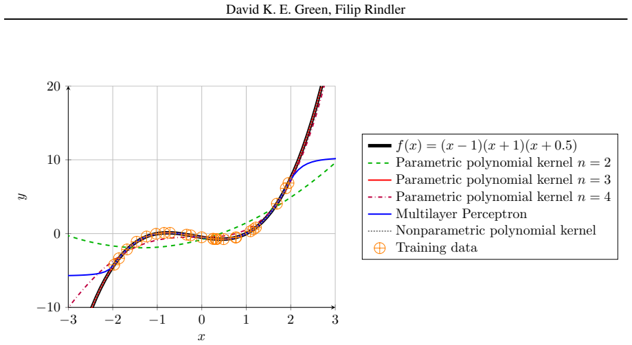
The central object is the parametric polynomial kernel: a compute graph (a directed graph of simple differentiable operations whose parameters are optimised by gradient descent) computing $f_\theta(u)=W_2\big[(W_1u+B_1)^{\circ n}\big]+B_2$, where the $\circ n$ superscript denotes an $n$-fold elementwise product. The first affine map projects the state $u$ into an $M$-dimensional intermediate representation whose entries are raised to the $n$th power, and the output layer blends those implicit monomial features into the vector field. This object carries the argument because it generates every polynomial coupling up to degree $n$ without ever writing the terms out, and because every operation is differentiable, so backpropagation can train it. The second load-bearing piece is the discretised ODE loss $\hat J_A(\theta)$, built from an Adams–Moulton step, which turns the integral of the unknown vector field into a differentiable function of $\theta$ that depends only on observed states.
What would settle it
Train the parametric polynomial kernel on Lorenz–Emanuel data exactly as described, then integrate the fitted model from a fresh initial condition in closed loop (using only its own predicted states) and record the time at which the accumulated error $\epsilon(t)$ exceeds a fixed threshold, say $1$. If that time is no longer than the training sampling interval, the long-horizon tracking claim fails; if it remains an order of magnitude longer, the claim survives.
Extended reading notes
Core claim
On the paper's own terms, the central claim is that a hidden polynomial ODE vector field can be recovered by replacing the support-vector expansion of kernel ridge regression with a fixed-parameter compute graph of the form $$f_\$\theta$(u)=W_2\big[(W_1u+B_1)\circ(W_1u+B_1)\big]+B_2$$ (or an $n$-fold elementwise product for higher degrees), and then optimising $\theta$ with stochastic gradient descent against a discretised integration loss. The first affine layer followed by the elementwise product plays the role of the polynomial kernel evaluation, and the output layer plays the role of the support-vector weights, so all polynomial couplings up to the chosen degree are represented implicitly. Inserting this function into an Adams–Moulton step gives a differentiable loss $\hat J_A(\theta)$, and backpropagation supplies the gradients. In the Lorenz–Emanuel experiments the accumulated error stayed small for times at least an order of magnitude longer than the sampling interval, larger intermediate dimensions $M$ improved accuracy, and the paper claims this recovers a maximum-likelihood estimate of the hidden polynomial model.
Load-bearing premise
The method's long-horizon tracking rests on the assumption that a model trained one step at a time against observed states will stay accurate when its own predictions are fed back for many integration steps; a separate load-bearing assumption, acknowledged in the paper, is that the true polynomial order is known in advance.
Editorial extensions
If this is right
- Any polynomial vector field of the chosen degree can be fitted this way, so the method is not tied to the Lorenz–Emanuel example; the kernel representation is agnostic to the number of state variables.
- Because the parameter count is fixed and each SGD step touches only the model and a minibatch of integration steps, training on very long time series avoids the cubic cost of inverting a kernel matrix.
- The fitted model is an explicit polynomial vector field, so it can be handed to any standard ODE solver for prediction, which the paper supports by testing with a different integrator than the one used in training.
- Increasing the intermediate dimension $M$ improves long-horizon accuracy at the cost of training time, providing a direct accuracy–cost control for practitioners.
Reading between the lines
- The paper validates its model by comparing one-step-ahead predictions against observed states, but never by feeding the model's own predicted states back through its vector field; a closed-loop rollout test would substantially strengthen the long-horizon tracking claim.
- Because the authors cite streaming data and Bayesian filtering as motivation but do not test either, a natural extension is to run this regressor online with incremental updates or to use the inferred polynomial as the forward model in a particle filter; nothing in the method prevents either.
- The finding that direct polynomial projection underperforms the kernel form suggests the same representation could serve as a cheap surrogate for polynomial chaos expansions in uncertainty quantification, where explicit high-degree polynomial bases are the standard bottleneck.
Signed reviews
Editorial analysis
A structured set of objections, weighed in public.
Referee Report
Summary. The paper proposes a parametric polynomial kernel representation of the right-hand side of an ODE, trained with SGD/backpropagation on a discretized loss derived from numerical integration of observed trajectories. The training objective is constructed in Section 4.4 by inserting observed state values at every integration step, and the method is tested on a scalar cubic regression problem and on inference of the Lorenz-Emanuel system, where it is compared with a direct polynomial feature expansion and with ANNs. The authors claim that the inferred model tracks the chaotic system over horizons much longer than the training data sampling interval.
Significance. The proposed representation is a sensible way to combine polynomial-kernel expressiveness with parametric scalability, and the derivation of the discretized loss is coherent and clearly presented. The simple regression example usefully demonstrates that the parametric polynomial kernel extrapolates better than a multilayer perceptron, and the Lorenz-Emanuel experiment shows that the model can fit an in-class quadratic vector field. The main weakness is that the central long-horizon tracking claim is not supported by the current experimental design: training minimizes a teacher-forced local loss, while evaluation measures autonomous rollout error, and only a single run appears to be reported. If the missing closed-loop validation and multi-seed statistics are supplied, the method would be a useful contribution to model inference for ODEs.
major comments (3)
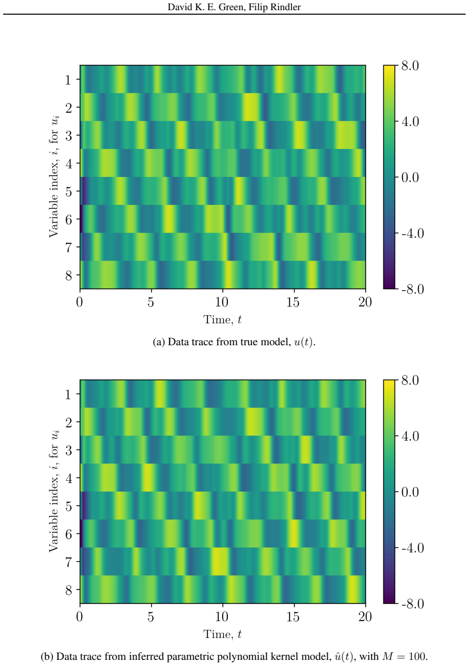
- [Section 4.4, Eqs. (37)-(40)] The training loss J_hat(theta) is teacher-forced: each prediction step starts from the observed u(t_i) and evaluates f_theta at observed points u(tau_j), so the objective penalizes only one- or two-step-ahead local error. In Section 5.4, however, the inferred model is evaluated by integrating it autonomously from new initial conditions (Fig. 6), which is precisely the regime not controlled by the training objective. The paper offers no closed-loop training and no stability or error-propagation analysis; Section 5.5 explicitly defers such analysis as beyond the scope. The abstract's claim of tracking 'over time periods much larger than the training data sampling rate' therefore rests on an unverified assumption. The authors should either train with closed-loop/unrolled trajectories, provide a rigorous argument that minimizing the teacher-forced loss controls the autonomous rollout, or re-scope the claim to short-horizon local prediction.
- [Section 5.2 and Fig. 6] No repeated runs, error bars, or confidence intervals are reported. Only a single training trajectory and a single SGD run per configuration appear to be used, although the system is chaotic and SGD is stochastic. The observed tracking in Fig. 6 may therefore not be representative. The paper should report statistics over multiple random initial conditions and optimizer seeds, and state explicitly how many trajectories and repeated training runs were used.
- [Sections 5.3 and 6] The Lorenz-Emanuel demonstration is an in-class fitting problem: the true vector field in Eq. (50) is quadratic, and the model class is restricted to second-order polynomials in Eqs. (13) and (54). While the exact coefficients are not provided to the optimizer, the paper acknowledges in Section 6 that the polynomial order is assumed known a priori and that using the wrong order causes convergence difficulties. The experiment therefore supports calibration of a known parametric family more than it supports the general model-inference claims made in Sections 1 and 6. An out-of-class experiment (e.g., a non-polynomial or noisy system, or an order-selection procedure) or an explicit restriction of the claims is needed.
minor comments (5)
- [Section 1] The statement that the method 'is able to recover a maximum likelihood estimate of the hidden polynomial model' is unsupported, because no likelihood or noise model is defined; the objective in Eq. (40) is a deterministic least-squares loss. Recommend replacing this phrase with 'least-squares estimate' or introducing an explicit probabilistic model.
- [Abstract and Section 5.4] The phrase 'time periods much larger than the training data sampling rate' is ambiguous and appears inconsistent with the more modest statement in Section 5.4 that errors are small 'at least an order of magnitude greater than the training data sampling rate.' If the sampling interval is h=0.001, an order of magnitude greater is about 0.01 time units; the paper should quantify the horizon in absolute time units and use consistent terminology.
- [Eq. (13)] The dimensions appear inconsistent: W1 is in R^{M x D}, so W1x is in R^M, and the bias B1 should therefore lie in R^M rather than R^D as stated.
- [Eq. (56)] The accumulated error is not fully specified: it should state the norm used over the eight state variables and clarify whether the recurrence accumulates squared errors under the final square root, since the current notation is ambiguous.
- [Fig. 6] The figure uses logarithmic axes but does not mark the sampling interval or the threshold used to define 'small error.' Adding a vertical line at the sampling interval and a legend or caption statement defining the small-error criterion would help the reader interpret the tracking claim.
Circularity Check
No significant circularity: the derivation is self-contained, and the in-class polynomial fit is an explicitly acknowledged modeling assumption rather than a prediction forced by construction.
full rationale
The paper's chain from the parametric polynomial representation (Eq. 13) through the discretized loss (Eqs. 37-40) to the Lorenz-Emmanuel experiments is internally consistent and does not reduce to its own inputs. The strongest candidate for circularity is that the model class is chosen to contain the true quadratic dynamics: Eq. 13 is a second-order polynomial in the state variables, while Eq. 50 is quadratic. That is a modeling assumption, not a derivation of the target from itself. The paper explicitly acknowledges this: Section 6 states 'It was assumed for the analysis in this paper that it was known a priori that only certain polynomial couplings are present.' This is a limitation, not a circular step. A second candidate is the teacher-forced loss in Eq. 40, which inserts observed values u(t_i) and u(tau_j) at each integration step. Minimizing this one-step-ahead loss does not, by construction, guarantee that the autonomous rollout of the trained vector field remains accurate; but the paper does not claim the loss forces that outcome. The long-horizon behavior is instead an empirical claim, tested in Section 5.2 by 'resampling new initial conditions' and comparing generated simulations against the true model. The lack of closed-loop training or stability analysis is a robustness gap, not a circularity. No load-bearing self-citation appears: the references to Sprott (Eq. 50), Sudret (Eq. 54), and standard integration/optimization texts are external background. The phrase 'recover a maximum likelihood estimate' in Section 1 is unsupported because no likelihood is defined, but this is an overclaim about statistical interpretation, not a reduction of the result to its inputs. Since every load-bearing step is either an explicit ansatz, a standard discretization, or an empirical evaluation on fresh initial conditions, the paper is not circular.
Assumptions & free parameters
free parameters (3)
- M (intermediate representation dimension) =
60, 80, 100 (tuned)
- polynomial order n =
3 (true order) for the cubic example; 2 for Lorenz-Emanuel
- training schedule (I_i, eta_i) =
P1=(1000,0.1), P2=(2000,0.01), P3=(200,0.001)
assumptions (4)
- domain assumption The system dynamics can be represented exactly as a polynomial of known order
- domain assumption Observations are noiseless
- domain assumption A one-step teacher-forcing loss is a valid proxy for multi-step prediction
- domain assumption Numerical integration at the training data sampling rate is sufficiently accurate
Cite this review
Pith. "Pith review of Model inference for Ordinary Differential Equations by parametric polynomial kernel regression." pith.science (2026). https://pith.science/paper/7646IOLJ
@misc{pith2026190802105,
  author       = {Pith},
  title        = {Pith review of: Model inference for Ordinary Differential Equations by parametric polynomial kernel regression},
  year         = {2026},
  howpublished = {\url{https://pith.science/paper/7646IOLJ}},
  note         = {Machine review of arXiv:1908.02105}
}
read the original abstract
Model inference for dynamical systems aims to estimate the future behaviour of a system from observations. Purely model-free statistical methods, such as Artificial Neural Networks, tend to perform poorly for such tasks. They are therefore not well suited to many questions from applications, for example in Bayesian filtering and reliability estimation. This work introduces a parametric polynomial kernel method that can be used for inferring the future behaviour of Ordinary Differential Equation models, including chaotic dynamical systems, from observations. Using numerical integration techniques, parametric representations of Ordinary Differential Equations can be learnt using Backpropagation and Stochastic Gradient Descent. The polynomial technique presented here is based on a nonparametric method, kernel ridge regression. However, the time complexity of nonparametric kernel ridge regression scales cubically with the number of training data points. Our parametric polynomial method avoids this manifestation of the curse of dimensionality, which becomes particularly relevant when working with large time series data sets. Two numerical demonstrations are presented. First, a simple regression test case is used to illustrate the method and to compare the performance with standard Artificial Neural Network techniques. Second, a more substantial test case is the inference of a chaotic spatio-temporal dynamical system, the Lorenz--Emanuel system, from observations. Our method was able to successfully track the future behaviour of the system over time periods much larger than the training data sampling rate. Finally, some limitations of the method are presented, as well as proposed directions for future work to mitigate these limitations.
Figures


Figures from the paper (4 more)


Reference graph
Works this paper leans on
- [1]
- [2]
-
[3]
Bishop, Neural Networks for Pattern Recognition
C.M. Bishop, Neural Networks for Pattern Recognition. Oxford University Press, 1995
work page 1995
-
[4]
B. Carpenter, M.D. Hoffman, M. Brubaker, D. Lee, P. Li, M. Betancourt, The Stan math library: Reverse-mode automatic differentiation in C++. ArXiv, arXiv:1509.07164, 2015
arXiv 2015
-
[5]
R. Dormand, P.J. Prince, A family of embedded Runge-Kutta formulae, Journal of Com- putational and Applied Mathematics. 6(1), 19–26, 1980
work page 1980
-
[6]
P. Eberhard, C. Bischof, Automatic differentiation of numerical integration algorithms, Neural Networks. 68, 717–732, 1999
work page 1999
-
[7]
Epp, Discrete Mathematics with Applications
S. Epp, Discrete Mathematics with Applications. Cengage Learning, 2010
work page 2010
- [8]
Show all 29 references
-
[9]
Hager, Updating the Inverse of a Matrix, SIAM Review, 31(2), 221–239, 1989
W.W. Hager, Updating the Inverse of a Matrix, SIAM Review, 31(2), 221–239, 1989
1989
-
[10]
Hairer, S.P
E. Hairer, S.P. Nørsett, G. Wanner Solving Ordinary Differential Equations I: Nonstiff problems. Springer Science & Business Media, 1993
1993
-
[11]
Hairer, S.P
E. Hairer, S.P. Nørsett, G. Wanner Solving Ordinary Differential Equations II: Stiff and Differential-Algebraic Problems. Springer Science & Business Media, 1996
1996
-
[12]
Horn, C.R
R.A. Horn, C.R. Johnson, Matrix Analysis. Cambridge University Press, 2012
2012
-
[13]
Iserles, A First Course in the Numerical Analysis of Differential Equations
A. Iserles, A First Course in the Numerical Analysis of Differential Equations. Cambridge University Press, 2009
2009
-
[14]
Jones, T
E. Jones, T. Oliphant, P. Peterson, SciPy: Open source scientific tools for Python. http: //www.scipy.org/, 2018
2018
-
[15]
Kingma, J
D.P. Kingma, J. Ba, Adam: A Method for Stochastic Optimization, Proceedings of the 3rd International Conference on Learning Representations (ICLR). Springer Verlag, 2015
2015
-
[16]
Matthies, E
H.G. Matthies, E. Zander, B.V . Rosi `c, A. Litvinenko, O. Pajonk, Inverse Problems in a Bayesian Setting, Computational Methods for Solids and Fluids. 41, 245–286, 2016
2016
-
[17]
Meiss, Differential Dynamical Systems, Revised Edition
J.D. Meiss, Differential Dynamical Systems, Revised Edition. SIAM, 2017
2017
-
[18]
Murphy, Machine Learning: A Probabilistic Perspective
K.P. Murphy, Machine Learning: A Probabilistic Perspective. MIT Press, 2012
2012
-
[19]
Pedregosa, G
F. Pedregosa, G. Varoquaux, A. Gramfort, V . Michel, B. Thirion, O. Grisel, M. Blondel, P. Prettenhofer, R. Weiss, V . Dubourg, J. Vanderplas, A. Passos, D. Cournapeau, M. Brucher, M. Perrot, E. Duchesnay, Scikit-learn: Machine Learning in Python, Journal of Machine Learning R...
2011
-
[20]
Rall, Automatic Differentiation: Techniques and Applications,Lecture Notes in Com- puter Science
L.B. Rall, Automatic Differentiation: Techniques and Applications,Lecture Notes in Com- puter Science. 120, 1981
1981
-
[21]
Russell, P
S. Russell, P. Norvig, Artificial Intelligence: A Modern Approach. Pearson, 2016
2016
-
[22]
Schmidt, H
M. Schmidt, H. Lipson, Distilling free-form natural laws from experimental data, Science. 324, 81–85, 2009
2009
-
[23]
Sprott, Elegant Chaos: Algebraically Simple Chaotic Flows
J.C. Sprott, Elegant Chaos: Algebraically Simple Chaotic Flows . World Scientific Pub- lishing Company, 2010
2010
-
[24]
Stanley, R
K.O. Stanley, R. Miikkulainen, Evolving Neural Networks through Augmenting Topolo- gies, Evolutionary Computation. 10(1), 99–127, 2002
2002
-
[25]
Stuart, Inverse problems: A Bayesian perspective, Acta Numerica
A.M. Stuart, Inverse problems: A Bayesian perspective, Acta Numerica. 19, 451–559, 2005
2005
-
[26]
B. Sudret, Uncertainty propagation and sensitivity analysis in mechanical models: Con- tributions to structural reliability and stochastic spectral methods , Habilitation `a diriger des recherches, Universit´e Blaise Pascal, 2007
2007
-
[27]
Taylor, Classical Mechanics
J.R. Taylor, Classical Mechanics. University Science Books, 2005
2005
-
[28]
K. Vu, J.C. Snyder, L. Li, M. Rupp, B.F. Chen, T. Khelif, K.R. M ¨uller, K. Burke, Un- derstanding kernel ridge regression: Common behaviors from simple functions to density functionals, International Journal of Quantum Chemistry. 115(16), 1115–1128, 2015
2015
-
[29]
Werbos, Generalisation of Backpropagation with application to a recurrent gas market model, Neural Networks
P. Werbos, Generalisation of Backpropagation with application to a recurrent gas market model, Neural Networks. 1(4), 339–356, 1988. 23
1988
Reviewed August 14, 2026 · model on record in the stance chip above.
Discussion (0). Continue with ORCID to comment.