REVIEW 2 major objections 4 minor 49 references
Bayesian Batch Active Learning as Sparse Subset Approximation
T0 review · 2 major / 4 minor · reviewed 2026-08-14 · deepseek-v4-flash
Pith's one-line read The paper frames batch active learning as sparse subset approximation of the expected complete-data log-posterior and shows that Frank-Wolfe optimization of this objective builds diverse, scalable query batches.
desk verdict A genuinely useful application of Hilbert coresets to batch active learning, with solid experiments and nice closed forms, but the 'principled' motivation rests on an unproven transfer assertion that the paper should either prove or soften. read the letter →
The pith
A machine-rendered reading of the paper's core claim, the machinery that carries it, and where it could break.
The reading
What carries the argument
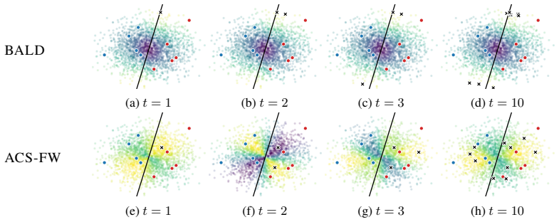
The load-bearing object is the set of expected log-likelihood functions $L_m$ viewed as vectors in a function space with an inner product. The weighted Fisher inner product $\langle L_n, L_m \rangle_{\hat{\pi},F} = \mathbb{E}_{\hat{\pi}}[\nabla_\theta L_n(\theta)^T \nabla_\theta L_m(\theta)]$ gives closed-form interpretable acquisition scores for linear and probit models; the weighted Euclidean inner product $\mathbb{E}_{\hat{\pi}}[L_n(\theta) L_m(\theta)]$ only requires likelihood evaluations and can be estimated by random projections $\hat{L}_n = J^{-1/2}[L_n(\theta_1),\dots,L_n(\theta_J)]^T$ with $\theta_j \sim \hat{\pi}$. The Frank-Wolfe algorithm does the work of batch construction: at each iteration it selects the vertex of the polytope most aligned with the residual $L - L(w)$, then updates weights by line search, so the batch is built by diversity-promoting residual matching rather than by thresholding a fixed acquisition score.
What would settle it
On a small regression problem where the full posterior is computable, run ACS-FW and a random batch of the same size, compute the posterior divergence between the batch-updated posterior and the complete-data posterior, and record $\|L - L(w)\|$ for both. If the random batch achieves as small a posterior divergence for a comparable function-space error, or if lower function-space error does not track lower posterior divergence, the motivating transfer claim is refuted.
Extended reading notes
Core claim
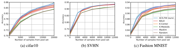
The central discovery is that the acquisition problem, which unlabeled points to label next, can be written as minimizing $\|L - L(w)\|$ in a Hilbert space, where $L_m(\theta) = \mathbb{E}_{y_m}[\log p(y_m \mid x_m, \theta)] + H[y_m \mid x_m, D_0]$ and $L = \sum_m L_m$ is the expected full-pool log-likelihood under the current predictive posterior. Relaxing the binary selection vector $w$ to nonnegative weights on the polytope $\{w : w_m \ge 0,\ \sum_m w_m \sigma_m = \sigma\}$ turns batch construction into a convex quadratic program that Frank-Wolfe solves by repeatedly adding the pool point whose log-likelihood vector is most aligned with the current residual. For linear regression the method yields the closed-form inner product $x_n^T x_m \sigma_0^{-4} x_n^T \Sigma_\theta x_m$, connecting the greedy version to BALD and to leverage scores; for probit regression the closed form uses the bivariate Normal cdf and Owen's T function. For arbitrary models, $J$ random projections of the log-likelihood terms give an unbiased estimator of the Euclidean inner product, making the per-iteration cost linear in the pool size. Experiments on UCI regressions, CIFAR-10, SVHN, and Fashion MNIST show ACS-FW matching or exceeding existing batch methods and consistently beating random selection.
Load-bearing premise
The load-bearing premise is that a small approximation error in the expected complete-data log-posterior implies the corresponding batch posterior is close to the full-data posterior; the paper asserts this link but provides no theorem or bound for it.
Editorial extensions
If this is right
- ACS-FW constructs batches that avoid the correlated queries of MAXENT and BALD, because the acquisition direction rotates after each selected point.
- With random projections, batch construction runs in $O(|P| J)$ time, so the method scales to pools of hundreds of thousands of points.
- On UCI regressions, CIFAR-10, SVHN, and Fashion MNIST, ACS-FW consistently beats random selection and performs at least as well as non-probabilistic batch AL baselines such as K-Center and K-Medoids.
- For linear models, the greedy version of the acquisition score is proportional to BALD up to an input-magnitude factor, making the method a direct extension of existing information-theoretic AL.
- The paper claims this provides a scalable, model-agnostic Bayesian batch active learning algorithm that does not require retraining after every single query.
Reading between the lines
- Editorial inference: the function-space objective is only a proxy; without a transfer bound between $\|L - L(w)\|$ and posterior divergence, the theoretical motivation could fail even if the algorithm works. Plugging in a coreset-style bound would be the natural repair.
- Editorial inference: the final binarization of Frank-Wolfe weights discards the fractional weights that line search computed; keeping continuous weights or using them for weighted retraining might improve the selected batch.
- Editorial inference: the inner product is a free design choice. Different kernels on $L_m$ would encode different notions of similarity between queries and could be tuned to a task, connecting the method to data geometry.
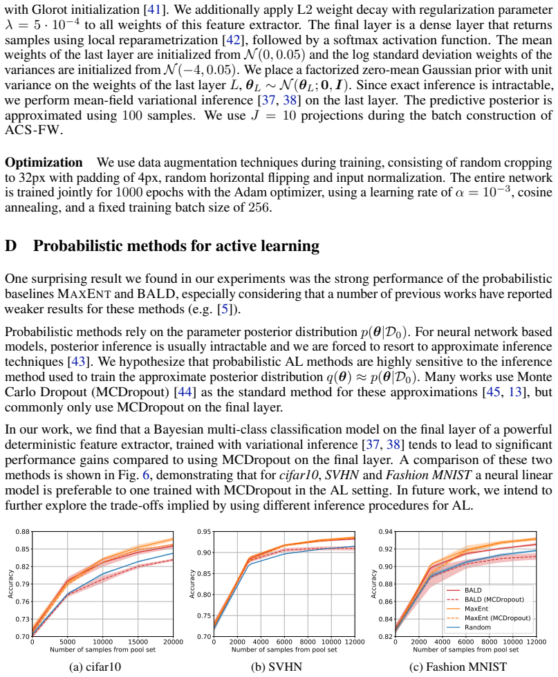
- Editorial inference: the appendix's observation that variational inference beats MC Dropout suggests the gains of ACS-FW on classification may depend as much on the inference procedure as on the batch algorithm; a controlled study varying only the inference method would isolate this.
Signed reviews
Editorial analysis
A structured set of objections, weighed in public.
Referee Report
Summary. The paper proposes ACS-FW, a Bayesian batch active learning method that constructs each batch by solving a sparse subset approximation to the expected complete-data log posterior. The objective is relaxed into a Hilbert-space norm minimization and solved with Frank-Wolfe, with closed-form inner products for Bayesian linear and probit regression, and a random-projection estimator of the Euclidean inner product for arbitrary tractable likelihoods. The authors compare ACS-FW against random selection, MAXENT, BALD, k-center, and k-medoids on UCI regression datasets, cifar10, SVHN, and Fashion MNIST, reporting that ACS-FW outperforms random selection and matches or exceeds existing batch methods, with favorable runtime scaling. The theoretical motivation is that a small function-space approximation error implies a close posterior, but no transfer bound is provided.
Significance. The paper offers a novel and elegant reformulation of batch active learning as sparse subset approximation of the expected complete-data log posterior, drawing on the Hilbert coreset toolbox. If the theoretical gap identified below can be closed, the method would provide a scalable, model-agnostic Bayesian alternative to existing batch AL heuristics. The closed-form connections to BALD and leverage scores for linear models, the random-projection extension to general likelihoods, and the empirical results on datasets with hundreds of thousands of points are the main strengths. The paper also releases source code, which supports reproducibility. However, the missing transfer guarantee between the approximation objective and the actual AL objective is a substantive caveat; the empirical gains over strong baselines such as MAXENT are real but modest on the small datasets.
major comments (2)
- [Section 3, Eqs. (4)-(6)] The paper's central claim that ACS-FW is a principled Bayesian batch AL method rests on the assertion in Section 3 that a good function-space approximation to L implies that the resulting posterior is close to the expected complete-data posterior. No theorem or bound is provided connecting ||L - L(w)|| to a divergence between p(θ|D0∪D') and p(θ|D0∪Dp), nor to the expected posterior entropy objective in Eq. (2). Because Eq. (4) targets the expectation of the log posterior while Eq. (2) is an expectation over posterior entropies with realized labels, even an exact optimizer of Eq. (5) would not automatically be near-optimal for the AL objective. Please add a quantitative transfer result (or a counterexample analysis) or explicitly re-frame the sparse-subset objective as a heuristic surrogate.
- [Section 5, Eqs. (9), (16)] For the weighted Euclidean inner product used in the random-projection variant, the constant entropy term H[y_m|x_m,D0] in L_m (Eq. (4)) does not vanish, since no gradient is taken. This term is irrelevant for the posterior, but it contributes to the norm and to the inner products estimated in Eq. (16), so the objective (5) may be dominated by label-independent constants. Please analyze how this affects the selected batch; if the entropy term is intended to be included, a justification is needed, and if not, it should be removed from L_m before projection.
minor comments (4)
- [Section 4, Eq. (12)] In Section 4 (Eq. (12)) and Appendix B.1, the statement that exp(2 α_BALD) is proportional to α_ACS is incorrect: exp(2 α_BALD) = 1 + x_n^T Σ_θ x_n / σ_0^2 (up to constants), which is affine rather than proportional to α_ACS without the x_n^T x_n factor. The conclusion that the two criteria have the same greedy maximizer is still correct because both are monotone in x_n^T Σ_θ x_n, but the proportionality claim should be corrected.
- [Section 3, after Algorithm 1] The sentence 'Empirically, we find that this property leads to smaller batches as more data points are acquired' is not supported by any experimental result in the paper; please provide evidence or remove the claim.
- [Appendix B.2] In Appendix B.2, the line after Eq. (20) writes Φ(ζ_m)Φ(ζ_m) where Φ(ζ_n)Φ(ζ_m) is intended; fix the typo.
- [Section 5, Experiments] The random-projection method in Section 5 uses J=10 throughout the experiments; since Eq. (17) is a Monte Carlo estimator, please report the sensitivity of the results to J or justify the choice.
Circularity Check
Derivation is self-contained; no circular reduction found.
full rationale
The paper's derivation chain starts from the expected complete-data log posterior (Eq. 4), defines the sparse-subset objective (Eq. 5), relaxes it to a Hilbert-space polytope problem (Eq. 6), and solves it with Frank-Wolfe. The selection weights are produced solely from inner products of the L_m vectors under the current posterior; none of these quantities are fitted to the test accuracies/RMSEs reported later, and those reported results are external benchmarks against RANDOM, BALD, MAXENT, K-CENTER, etc. The observation that the greedy norm α_ACS is proportional to BALD for linear regression (Section 4) is an equivalence to an existing acquisition function, not a circular use of that function to define the method. The only load-bearing caveat is the Section 3 assertion that approximating L implies a close posterior; that claim is stated without a transfer bound, but a missing proof is a correctness risk rather than circularity, since the objective is not defined in terms of the AL outcome it predicts. The single self-citation ([24], Hernández-Lobato & Adams) is contextual in the related-work discussion and does not support any step of the derivation.
Assumptions & free parameters
free parameters (1)
- J (number of random projections) =
10
assumptions (6)
- domain assumption Conditional independence of outputs given inputs, so that the expected log-likelihood sum factorizes over pool points.
- domain assumption The current posterior pi_hat = p(theta|D0) is a good basis for defining the expected complete-data log-posterior and for computing inner products.
- domain assumption The approximation sigma(z) approximately Phi(z) for probit/logistic regression.
- ad hoc to paper A small function-space error ||L - L(w)|| implies the resulting posterior is close to the expected complete-data posterior.
- standard math Frank-Wolfe converges sufficiently for the convex quadratic program in Eq. (6).
- domain assumption The random projection estimator in Eq. (16) is an unbiased, low-variance estimator of the Euclidean inner product at J=10.
Cite this review
Pith. "Pith review of Bayesian Batch Active Learning as Sparse Subset Approximation." pith.science (2026). https://pith.science/paper/YBV277XO
@misc{pith2026190802144,
  author       = {Pith},
  title        = {Pith review of: Bayesian Batch Active Learning as Sparse Subset Approximation},
  year         = {2026},
  howpublished = {\url{https://pith.science/paper/YBV277XO}},
  note         = {Machine review of arXiv:1908.02144}
}
read the original abstract
Leveraging the wealth of unlabeled data produced in recent years provides great potential for improving supervised models. When the cost of acquiring labels is high, probabilistic active learning methods can be used to greedily select the most informative data points to be labeled. However, for many large-scale problems standard greedy procedures become computationally infeasible and suffer from negligible model change. In this paper, we introduce a novel Bayesian batch active learning approach that mitigates these issues. Our approach is motivated by approximating the complete data posterior of the model parameters. While naive batch construction methods result in correlated queries, our algorithm produces diverse batches that enable efficient active learning at scale. We derive interpretable closed-form solutions akin to existing active learning procedures for linear models, and generalize to arbitrary models using random projections. We demonstrate the benefits of our approach on several large-scale regression and classification tasks.
Figures


Figures from the paper (3 more)

Reference graph
Works this paper leans on
-
[1]
Burr Settles. Active learning. Synthesis Lectures on Artificial Intelligence and Machine Learning, 6(1):1–114, 2012
work page 2012
-
[2]
Information-based objective functions for active data selection
David JC MacKay. Information-based objective functions for active data selection. Neural computation, 4(4):590–604, 1992
1992
-
[3]
A mathematical theory of communication
Claude Elwood Shannon. A mathematical theory of communication. Bell System Technical Journal, 27(3):379–423, 1948
work page 1948
-
[4]
Bayesian active learning for classification and preference learning
Neil Houlsby, Ferenc Huszár, Zoubin Ghahramani, and Máté Lengyel. Bayesian active learning for classification and preference learning. arXiv Preprint arXiv:1112.5745, 2011
arXiv 2011
-
[5]
Active learning for convolutional neural networks: A core-set approach
Ozan Sener and Silvio Savarese. Active learning for convolutional neural networks: A core-set approach. In International Conference on Learning Representations, 2018
2018
-
[6]
A convex optimization framework for active learning
Ehsan Elhamifar, Guillermo Sapiro, Allen Yang, and S Shankar Sasrty. A convex optimization framework for active learning. In IEEE International Conference on Computer Vision, pages 209–216, 2013
work page 2013
-
[7]
Active instance sampling via matrix partition
Yuhong Guo. Active instance sampling via matrix partition. In Advances in Neural Information Processing Systems, pages 802–810, 2010
work page 2010
-
[8]
Multi-class active learning by uncertainty sampling with diversity maximization
Yi Yang, Zhigang Ma, Feiping Nie, Xiaojun Chang, and Alexander G Hauptmann. Multi-class active learning by uncertainty sampling with diversity maximization. International Journal of Computer Vision, 113(2):113–127, 2015
work page 2015
Show all 49 references
-
[9]
Coresets for scalable Bayesian logistic regression
Jonathan Huggins, Trevor Campbell, and Tamara Broderick. Coresets for scalable Bayesian logistic regression. In Advances in Neural Information Processing Systems, pages 4080–4088, 2016
2016
-
[10]
Automated scalable Bayesian inference via Hilbert coresets
Trevor Campbell and Tamara Broderick. Automated scalable Bayesian inference via Hilbert coresets. The Journal of Machine Learning Research, 20(1):551–588, 2019
2019
-
[11]
An algorithm for quadratic programming
Marguerite Frank and Philip Wolfe. An algorithm for quadratic programming. Naval Research Logistics Quarterly, 3(1-2):95–110, 1956
1956
-
[12]
Visualizing data using t-SNE.Journal of Machine Learning Research, 9(Nov):2579–2605, 2008
Laurens van der Maaten and Geoffrey Hinton. Visualizing data using t-SNE.Journal of Machine Learning Research, 9(Nov):2579–2605, 2008
2008
-
[13]
Deep Bayesian active learning with image data
Yarin Gal, Riashat Islam, and Zoubin Ghahramani. Deep Bayesian active learning with image data. arXiv Preprint arXiv:1703.02910, 2017
2017 arXiv
-
[14]
Adaptive submodularity: Theory and applications in active learning and stochastic optimization
Daniel Golovin and Andreas Krause. Adaptive submodularity: Theory and applications in active learning and stochastic optimization. Journal of Artificial Intelligence Research , 42: 427–486, 2011
2011
-
[15]
Analysis of a greedy active learning strategy
Sanjoy Dasgupta. Analysis of a greedy active learning strategy. In Advances in Neural Information Processing Systems, pages 337–344, 2005
2005
-
[16]
Deep residual learning for image recognition
Kaiming He, Xiangyu Zhang, Shaoqing Ren, and Jian Sun. Deep residual learning for image recognition. In IEEE Conference on Computer Vision and Pattern Recognition, pages 770–778, 2016. 10
2016
-
[17]
Fisher information inequalities and the central limit theorem
Oliver Johnson and Andrew Barron. Fisher information inequalities and the central limit theorem. Probability Theory and Related Fields, 129(3):391–409, 2004
2004
-
[18]
Deep kernel learning
Andrew Gordon Wilson, Zhiting Hu, Ruslan Salakhutdinov, and Eric P Xing. Deep kernel learning. In Artificial Intelligence and Statistics, pages 370–378, 2016
2016
-
[19]
Deep Bayesian bandits showdown
Carlos Riquelme, George Tucker, and Jasper Snoek. Deep Bayesian bandits showdown. In International Conference on Learning Representations, 2018
2018
-
[20]
Fast approximation of matrix coherence and statistical leverage
Petros Drineas, Malik Magdon-Ismail, Michael W Mahoney, and David P Woodruff. Fast approximation of matrix coherence and statistical leverage. Journal of Machine Learning Research, 13(Dec):3475–3506, 2012
2012
-
[21]
A statistical perspective on algorithmic leveraging
Ping Ma, Michael W Mahoney, and Bin Yu. A statistical perspective on algorithmic leveraging. The Journal of Machine Learning Research, 16(1):861–911, 2015
2015
-
[22]
Leveraged volume sampling for linear regression
Michal Derezinski, Manfred K Warmuth, and Daniel J Hsu. Leveraged volume sampling for linear regression. In Advances in Neural Information Processing Systems, pages 2510–2519, 2018
2018
-
[23]
Tables for computing bivariate normal probabilities
Donald B Owen. Tables for computing bivariate normal probabilities. The Annals of Mathemat- ical Statistics, 27(4):1075–1090, 1956
1956
-
[24]
Probabilistic backpropagation for scalable learning of Bayesian neural networks
José Miguel Hernández-Lobato and Ryan Adams. Probabilistic backpropagation for scalable learning of Bayesian neural networks. In International Conference on Machine Learning, pages 1861–1869, 2015
2015
-
[25]
Active learning via transductive experimental design
Kai Yu, Jinbo Bi, and V olker Tresp. Active learning via transductive experimental design. In International Conference on Machine Learning, pages 1081–1088, 2006
2006
-
[26]
Batch mode active learning and its application to medical image classification
Steven CH Hoi, Rong Jin, Jianke Zhu, and Michael R Lyu. Batch mode active learning and its application to medical image classification. In International Conference on Machine Learning, pages 417–424, 2006
2006
-
[27]
Discriminative batch mode active learning
Yuhong Guo and Dale Schuurmans. Discriminative batch mode active learning. In Advances in Neural Information Processing Systems, pages 593–600, 2008
2008
-
[28]
Submodularity in data subset selection and active learning
Kai Wei, Rishabh Iyer, and Jeff Bilmes. Submodularity in data subset selection and active learning. In International Conference on Machine Learning, pages 1954–1963, 2015
1954
-
[29]
Fast computation of the multi-points expected improvement with applications in batch selection
Clément Chevalier and David Ginsbourger. Fast computation of the multi-points expected improvement with applications in batch selection. In International Conference on Learning and Intelligent Optimization, pages 59–69, 2013
2013
-
[30]
Parallel predictive entropy search for batch global optimization of expensive objective functions
Amar Shah and Zoubin Ghahramani. Parallel predictive entropy search for batch global optimization of expensive objective functions. In Advances in Neural Information Processing Systems, pages 3330–3338, 2015
2015
-
[31]
Batch Bayesian optimization via simulation matching
Javad Azimi, Alan Fern, and Xiaoli Z Fern. Batch Bayesian optimization via simulation matching. In Advances in Neural Information Processing Systems, pages 109–117, 2010
2010
-
[32]
Parallel gaussian process optimization with upper confidence bound and pure exploration
Emile Contal, David Buffoni, Alexandre Robicquet, and Nicolas Vayatis. Parallel gaussian process optimization with upper confidence bound and pure exploration. In Joint European Conference on Machine Learning and Knowledge Discovery in Databases , pages 225–240, 2013
2013
-
[33]
Parallelizing exploration-exploitation tradeoffs in gaussian process bandit optimization
Thomas Desautels, Andreas Krause, and Joel W Burdick. Parallelizing exploration-exploitation tradeoffs in gaussian process bandit optimization. The Journal of Machine Learning Research, 15(1):3873–3923, 2014
2014
-
[34]
Batch Bayesian optimiza- tion via local penalization
Javier González, Zhenwen Dai, Philipp Hennig, and Neil Lawrence. Batch Bayesian optimiza- tion via local penalization. In Artificial Intelligence and Statistics, pages 648–657, 2016. 11
2016
-
[35]
Active learning with Gaussian processes for object categorization
Ashish Kapoor, Kristen Grauman, Raquel Urtasun, and Trevor Darrell. Active learning with Gaussian processes for object categorization. In IEEE International Conference on Computer Vision, pages 1–8, 2007
2007
-
[36]
Adam: A method for stochastic optimization
Diederik P Kingma and Jimmy Ba. Adam: A method for stochastic optimization. arXiv Preprint arXiv:1412.6980, 2014
2014 arXiv
-
[37]
Graphical models, exponential families, and variational inference
Martin J Wainwright, Michael I Jordan, et al. Graphical models, exponential families, and variational inference. Foundations and Trends® in Machine Learning, 1(1–2):1–305, 2008
2008
-
[38]
Weight uncertainty in neural networks
Charles Blundell, Julien Cornebise, Koray Kavukcuoglu, and Daan Wierstra. Weight uncertainty in neural networks. arXiv Preprint arXiv:1505.05424, 2015
2015 arXiv
-
[39]
Machine learning: A probabilistic perspective
Kevin P Murphy. Machine learning: A probabilistic perspective. MIT Press, 2012
2012
-
[40]
Pattern recognition and machine learning
Christopher M Bishop. Pattern recognition and machine learning. Springer, 2006
2006
-
[41]
Understanding the difficulty of training deep feedforward neural networks
Xavier Glorot and Yoshua Bengio. Understanding the difficulty of training deep feedforward neural networks. In International Conference on Artificial Intelligence and Statistics, pages 249–256, 2010
2010
-
[42]
Variational dropout and the local reparam- eterization trick
Durk P Kingma, Tim Salimans, and Max Welling. Variational dropout and the local reparam- eterization trick. In Advances in Neural Information Processing Systems, pages 2575–2583, 2015
2015
-
[43]
Bayesian learning for neural networks , volume 118
Radford M Neal. Bayesian learning for neural networks , volume 118. Springer Science & Business Media, 2012
2012
-
[44]
Dropout: A simple way to prevent neural networks from overfitting
Nitish Srivastava, Geoffrey Hinton, Alex Krizhevsky, Ilya Sutskever, and Ruslan Salakhutdinov. Dropout: A simple way to prevent neural networks from overfitting. The Journal of Machine Learning Research, 15(1):1929–1958, 2014
1929
-
[45]
Dropout as a Bayesian approximation: Representing model uncertainty in deep learning
Yarin Gal and Zoubin Ghahramani. Dropout as a Bayesian approximation: Representing model uncertainty in deep learning. In International Conference on Machine Learning, pages 1050–1059, 2016. 12 A Algorithms A.1 Active Bayesian coresets with Frank-Wolfe optimization (ACS-FW) Al...
2016
-
[46]
=N (θ;µθ, Σθ) (18) µθ = ( XTX +σ2 0I )−1 XTy Σθ =σ2 0 ( XTX +σ2 0I )−1 , and the predictive posterior is given by p(yn|xn,D0,σ 2
-
[47]
(19) Using this model, we can derive a closed-form term for the inner product in Eq
= ∫ θ p(yn|xn,θ)p(θ|D0,σ 2 0)dθ =N (yn;µT θxn,σ 2 0 +xT nΣθxn). (19) Using this model, we can derive a closed-form term for the inner product in Eq. (8), ⟨Ln,Lm⟩ˆπ,F = Eˆπ [ (∇θLn)T (∇θLm) ] = Eˆπ [( 1 σ2 0 (E[yn]−xT nθ)xn )T( 1 σ2 0 (E[ym]−xT mθ)xm )] = xT nxm σ4 0 E ˆπ [( µT...
-
[48]
(19), and in the third equality w.r.t
from Eq. (19), and in the third equality w.r.t. ˆπ =p(θ|D0,σ 2
-
[49]
from Eq. (18). Similarly, we obtain ⟨Ln,Ln⟩ˆπ,F = xT nxn σ4 0 ( xT nΣθxn ) . For this model, BALD [2, 4] can also be evaluated in closed form: αBALD(xn;D0) = H [ θ|D0,σ 2 0 ] − Ep(yn|xn,D0) [ H [ θ|xn,yn,D0,σ 2 0 ]] = 1 2 Eˆπ [ logσ2 0 +xT nΣθxn σ2 0 + σ2 0 + (µT θxn−θTxn)2 σ2...
2000
Reviewed August 14, 2026 · model on record in the stance chip above.
Discussion (0). Continue with ORCID to comment.