REVIEW 3 major objections 5 minor 1 cited by
Understanding the HERA Phase I receiver system with simulations and its impact on the detectability of the EoR delay power spectrum
T0 review · 3 major / 5 minor · reviewed 2026-08-14 · deepseek-v4-flash
Pith's one-line read HERA Phase I's own cables and dish-to-dish coupling delay the 100,000-fold suppression of the system response to 1400 ns, so foreground avoidance leaves line-of-sight wavenumbers below 0.7 h/Mpc contaminated.
desk verdict The qualitative result—mutual coupling dominates HERA Phase I system response at high delays—is solid and important, but the headline 0.7 h/Mpc threshold is an unvalidated extrapolation from a half-length strip; the paper still deserves serious peer review. read the letter →
The pith
A machine-rendered reading of the paper's core claim, the machinery that carries it, and where it could break.
The reading
What carries the argument
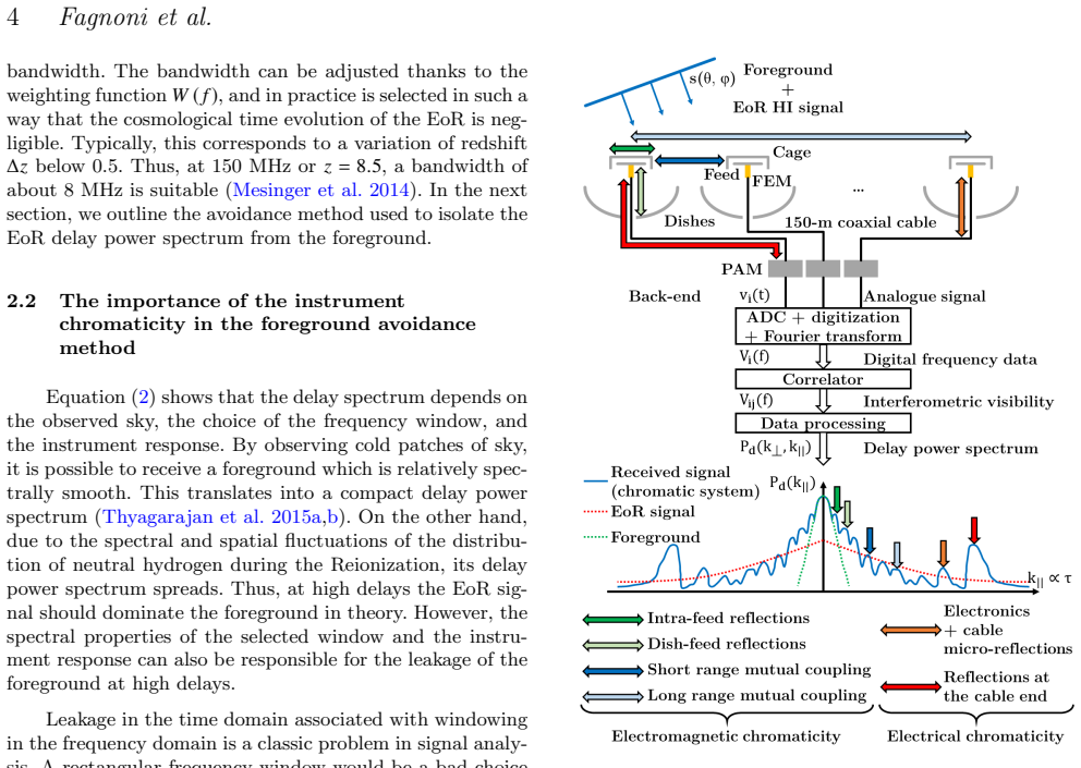
The load-bearing object is the system voltage time response $h(\tau)$, obtained by Fourier transforming $H(f)=V_2/E_{\mathrm{in}}$, where $V_2$ is computed from the antenna effective length and the receiver's two-port impedance matrix. Mutual coupling is included by terminating the $2N$-port array $Z$-matrix with the receiver impedance and solving for the input impedance seen by each antenna. A Blackman-Harris window over the 100-200 MHz band sets the $10^{-5}$ noise floor against which reflection levels are judged. The delay-to-wavenumber relation $k_\parallel = 2\pi f_{21} H_p(z)\,\tau/[c(1+z)^2]$ converts the 1400 ns delay into the $0.7\,h\,\mathrm{Mpc}^{-1}$ boundary at 150 MHz.
What would settle it
Take the autocorrelation visibility of an edge antenna in the deployed HERA core, Fourier transform to delay, and compare the envelope with the simulated response: if the normalized response falls below $10^{-5}$ before roughly 1000 ns, the extrapolated boundary is too pessimistic, and if it stays above $10^{-5}$ past 1400 ns, the boundary is too optimistic. A complementary check is to run the same electromagnetic simulation on a longer array and see whether the ~50 ns dish-to-dish echoes persist with the same decay slope.
Extended reading notes
Core claim
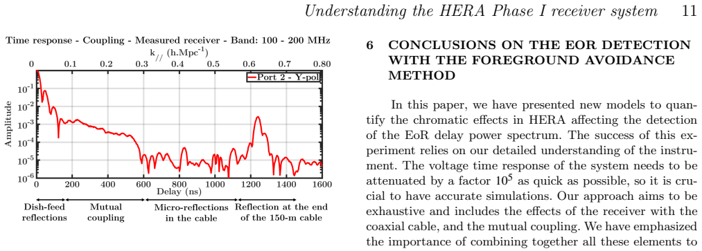
The central discovery is a four-regime system time response. At low delays, reflections between the feed cage and dish vertex dominate; in the mid-delay range, mutual coupling dominates, with echoes arriving roughly every 50 ns as waves hop from one 14.6-m dish to the next with little attenuation; then micro-reflections in the 150-m cable add a quasi-continuous floor; and finally the cable-end reflection produces a factor-300 bump around 1200-1300 ns. Extrapolating the mutual-coupling decay from the simulated 11-column strip to the 300-m core implies the overall response reaches $10^{-5}$ only near 1400 ns, corresponding to $k_\parallel\sim0.7\,h\,\mathrm{Mpc}^{-1}$ at 150 MHz, with edge antennas worse than central ones. The paper further establishes that the dominant coupling path is feed-dish scattering rather than direct feed-feed interaction, and that a source near the horizon can spread the response across a delay equal to twice the array crossing time.
Load-bearing premise
The simulation covers an 11-column strip about 150 m long and extrapolates the mutual-coupling decay slope to the full 300-m core; if echoes in the longer array die out faster or scatter differently, the 1400 ns / $0.7\,h\,\mathrm{Mpc}^{-1}$ boundary moves.
Editorial extensions
If this is right
- Under a strict foreground-avoidance analysis, HERA Phase I can only claim EoR delay power spectrum measurements at line-of-sight wavenumbers above about $0.7\,h\,\mathrm{Mpc}^{-1}$ at 150 MHz; modes below that are foreground-leakage contaminated.
- The usable wavenumber range is roughly a factor of 3.5 narrower than the earlier $0.2\,h\,\mathrm{Mpc}^{-1}$ threshold, cutting the number of clean line-of-sight modes available for the EoR measurement.
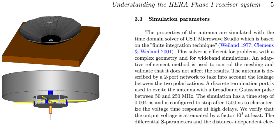
- Mutual coupling makes the system response depend on antenna position and array size, so edge antennas are more chromatic and the set of truly redundant baselines shrinks, complicating redundant-baseline calibration.
- Strong sources near the horizon are especially damaging: their geometric delay spread can reach twice the array crossing time, so horizon radio emission leaks into higher delays.
- Replacing the coaxial cable with optical links, as planned for Phase II, would remove the 1200-1300 ns cable-end reflection and the micro-reflection floor, leaving mutual coupling as the limiting chromatic effect.
Reading between the lines
- Inference: if the paper is right, the same coupled-array chromaticity will affect any close-packed 21-cm array whose dish spacing is comparable to a wavelength, so other EoR experiments should recheck their line-of-sight cutoffs with full-array mutual-coupling simulations rather than single-antenna responses.
- Inference: the array-size dependence implies a sensitivity-versus-chromaticity trade-off: bigger cores buy collecting area but push the foreground wall to larger delays; damping dish-rim scattering could recover some of that delay space.
- Inference: a direct test of the extrapolation is within reach: a long-duration autocorrelation measurement on the deployed array out to 1400 ns, or a simulation of the full core, would confirm or correct the 0.7 h/Mpc boundary before Phase I data are mined for cosmology.
- Inference: if the 1400 ns floor holds, Phase I's low line-of-sight modes will likely require calibration-based foreground subtraction or inverse-covariance weighting rather than avoidance, with avoidance reserved for the high-delay end.
Signed reviews
Editorial analysis
A structured set of objections, weighed in public.
Referee Report
Summary. The paper presents co-simulations of the HERA Phase I receiver system, combining electromagnetic models of the antenna array with circuit models of the receiver and cables, to quantify the instrument's chromatic response in the delay domain. It models internal reflections, cable micro-reflections, the 150-m cable end reflection, and mutual coupling in a reduced 11-column strip array. The central result is that the system voltage response is attenuated by only 10^5 after a delay of about 1400 ns, which the authors translate to a limiting k_parallel of about 0.7 h/Mpc at 150 MHz, implying that foreground avoidance with HERA Phase I is more challenging than previously estimated (which had suggested ~0.2 h/Mpc).
Significance. If the central claim holds, the paper is important: it directly affects the forecast sensitivity and data analysis strategy of HERA Phase I, a major 21-cm EoR experiment. The paper's strengths include validation of component models against VNA measurements, in-situ beam comparisons (to -20 dB), and receiver noise measurements; a clear separation of the contributions of different chromatic terms; and an explicit acknowledgement, in Section 5.3, that the full-core conclusion relies on an extrapolation of the decay slope from a reduced strip. The companion data paper (Kern et al. 2020a) provides partial empirical support to delay ~500 ns. The headline 1400 ns / 0.7 h/Mpc number, however, is not directly validated or simulated for the full core, so the quantitative significance is conditional on the validity of that extrapolation.
major comments (3)
- [Sec. 5.3 and Sec. 6] The headline quantitative claim that the system response is attenuated by 10^5 only after 1400 ns, and the resulting statement that k_parallel modes below 0.7 h/Mpc are affected, is not a direct simulation result for the full HERA core. Section 5.3 explicitly states that the simulated strip is 'half of the final length of the core' and that the 10^5 crossing at about 1000 ns is obtained by extrapolating the slope of the system response, with the 1400 ns figure then adding the 150-m cable reflection. The full core is a two-dimensional 300 m by 250 m array, not a doubled one-dimensional strip. Because this quantity is load-bearing for the paper's main conclusion, the extrapolation must be either validated (e.g., by a larger or full-core simulation, or by extending the empirical comparison to the relevant delay range) or presented with a quantitative uncertainty budget and clearly marked as an extrapolated estimate in the abstract and conclusions. Currently Section 6 states the 1400 ns and 0.7 h/Mpc values without this caveat.
- [Sec. 4.4 and Fig. 13] The mutual-coupling simulation is a one-dimensional 11-column strip with a specific edge termination. The conclusion that 'any antenna could significantly interact with the dishes at the edges' depends on the assumption that the dominant propagation path is along a single row and that the decay slope in the strip is representative of the full two-dimensional core. Equation (17) shows that the coupling delay depends on Dmax, which in a 2-D core would vary with direction and antenna position, and corner geometries or diagonal paths could modify the tail of the response. This assumption is not tested, yet it directly sets the time constant of the 10^-4 and 10^-5 crossings used in the paper. Please provide additional justification or a test of this strip-to-core extrapolation, or soften the full-core claims accordingly.
- [Sec. 6, last paragraph] The comparison with the 46-antenna data from Kern et al. (2020a) is described as 'consistent' with the simulations, but the data exhibit a noise floor at about 10^-4 after 500 ns. The decisive quantity for the headline claim is the 10^-5 crossing at about 1400 ns, which is not probed by these data. The paper should state explicitly the range of delays over which the simulations are empirically validated, and identify what evidence (if any) bears on the extrapolated regime. Without this, the statement in the abstract that 'the system response is attenuated by a factor 10^5 after 1400 ns' overstates the current level of validation.
minor comments (5)
- [Sec. 4.2, last paragraph] The sentence 'Nunhokee et al. (2020) has measured the HERA radiation pattern...' should use the plural verb 'have measured'.
- [Fig. 13 caption] The caption 'for various antenna configurations' is vague; please specify which positions (center, edge) and which configurations (all feeds present, single feed, etc.) are shown so the figure is self-contained.
- [Sec. 3.3] The statement 'We verify that the output voltage is attenuated by a factor 10^5 at least' should identify the configuration for which this verification was performed (single antenna versus array), since the later array simulations show a slower decay.
- [Eq. (17)] Please define Dmax explicitly as the distance to the farthest aligned antenna in the simulated strip, and note that for the full two-dimensional core this quantity would depend on direction and reference antenna position.
- [Sec. 5.3] The conditional sentence beginning 'If the simulated antenna strip were longer, the extrapolation of the slope...' is a key caveat. Consider moving this caveat to the abstract or conclusions, or at least ensuring the numbers quoted in Section 6 are clearly labeled as extrapolated estimates.
Circularity Check
No significant circularity: the simulated 1400 ns / 0.7 h Mpc^-1 threshold is an output of electromagnetic and circuit simulations whose inputs are external component measurements and a standard delay-to-k_parallel conversion, not a fit or self-referential derivation.
full rationale
The central claim, stated in Section 6 as "The response is attenuated by a factor 10^5 only after 1400 ns, which means that the k_parallel-modes below 0.7 h Mpc^-1 are affected by the foreground leakage," is a simulated output rather than a fitted parameter. The inputs are external component characterizations: CST antenna models, VNA measurements of receiver and cable S/Z parameters, manufacturer transistor data, and a literature-based sky model. No parameter is fitted to the EoR delay power spectrum or to the 10^5 crossing time. The 0.7 h Mpc^-1 value follows from the standard cosmological mapping in Equation (5), which converts delay tau to k_parallel using known redshift and bandwidth relations; it is not an assumption that contains the conclusion. The 10^5 attenuation requirement is stated as a foreground-contrast design goal, not derived from the simulation target. The paper also cites companion papers by collaboration members, notably Kern et al. (2020a) for 46-antenna data consistency and Kern et al. (2020b) for calibration applications, but the central prediction does not reduce to those citations: the measured data are presented as a consistency check with an explicitly acknowledged noise floor at about 10^-4 after 500 ns, and the simulation's delay tail is the primary evidence. The most significant limitation is the explicit extrapolation from the simulated 11-column strip, which is about half the final core length: Section 5.3 states "If the simulated antenna strip were longer, the extrapolation of the slope of the system response suggests..." and Section 6 notes the 46-antenna data were collected "in a larger two-dimensional array with a more complex configuration compared with our simulation." This is a transparent robustness and validation caveat about extrapolation, not a circular step: the conclusion is not equivalent to its inputs by construction, and no fitted input is renamed as a prediction. No uniqueness theorem is invoked, no ansatz is smuggled in via citation, and no known result is merely renamed. The main residual concern is correctness risk from extrapolating the mutual-coupling tail to the full core, not circularity.
Assumptions & free parameters
free parameters (4)
- Sky temperature power-law normalization =
180 K at 180 MHz
- Sky temperature spectral index =
-2.6
- Chromatic cable micro-reflection parameters =
Not reported
- Receiver noise parameters =
Fmin 1.6-1.8 dB, RN 27 ohm, Zopt 135+30j ohm
assumptions (4)
- domain assumption The antenna and receiver form a linear, time-invariant system, so the output voltage is a convolution of the incident field with an impulse response (Sec 2.1).
- domain assumption Far-field approximation for the antenna effective length, neglecting the radial field component (Sec 4.3, Eq. 10).
- domain assumption Uniform sky brightness for the system temperature estimate (Sec 5.1).
- ad hoc to paper The mutual coupling simulation strip is representative of the full HERA core, and the decay slope can be extrapolated to the full 300-m array (Sec 5.3, Fig. 13).
Cite this review
Pith. "Pith review of Understanding the HERA Phase I receiver system with simulations and its impact on the detectability of the EoR delay power spectrum." pith.science (2026). https://pith.science/paper/C6IHJX3S
@misc{pith2026190802383,
  author       = {Pith},
  title        = {Pith review of: Understanding the HERA Phase I receiver system with simulations and its impact on the detectability of the EoR delay power spectrum},
  year         = {2026},
  howpublished = {\url{https://pith.science/paper/C6IHJX3S}},
  note         = {Machine review of arXiv:1908.02383}
}
abstract
The detection of the Epoch of Reionization (EoR) delay power spectrum using a "foreground avoidance method" highly depends on the instrument chromaticity. The systematic effects induced by the radio-telescope spread the foreground signal in the delay domain, which contaminates the EoR window theoretically observable. Applied to the Hydrogen Epoch of Reionization Array (HERA), this paper combines detailed electromagnetic and electrical simulations in order to model the chromatic effects of the instrument, and quantify its frequency and time responses. In particular, the effects of the analogue receiver, transmission cables, and mutual coupling are included. These simulations are able to accurately predict the intensity of the reflections occurring in the 150-m cable which links the antenna to the back-end. They also show that electromagnetic waves can propagate from one dish to another one through large sections of the array due to mutual coupling. The simulated system time response is attenuated by a factor $10^{4}$ after a characteristic delay which depends on the size of the array and on the antenna position. Ultimately, the system response is attenuated by a factor $10^{5}$ after 1400 ns because of the reflections in the cable, which corresponds to characterizable ${k_\parallel}$-modes above 0.7 $h\;\rm{Mpc}^{-1}$ at 150 MHz. Thus, this new study shows that the detection of the EoR signal with HERA Phase I will be more challenging than expected. On the other hand, it improves our understanding of the telescope, which is essential to mitigate the instrument chromaticity.
Figures

Figures from the paper (11 more)




Forward citations
Cited by 1 Pith paper
-
Intensity fluctuations of radio halo in galaxy cluster: Insights from power spectrum estimation
Angular power spectra of 610 MHz radio halos show excess power-law fluctuations only in Abell 2744, requiring multiplicative C_ℓ ∝ ℓ^{-3} structure atop an exponential profile and consistent with ICM turbulence.
Reference graph
Works this paper leans on
-
[1]
S., et al., 2015, @doi [ApJ] 10.1088/0004-637X/809/1/61 , 809, 61
Ali Z. S., et al., 2015, @doi [ApJ] 10.1088/0004-637X/809/1/61 , 809, 61
-
[2]
Bowman J. D., Morales M. F., Hewitt J. N., 2009, @doi [ApJ] 10.1088/0004-637X/695/1/183 , 695, 183
-
[3]
Antennas Propag.] 10.1109/TAP.1981.1142671 , 29, 773
Bucci O., Di Massa G., Savarese C., 1981, @doi [IEEE Trans. Antennas Propag.] 10.1109/TAP.1981.1142671 , 29, 773
-
[4]
CEL 2012, NE461M02 / 2SC5337 NPN RF transistor data sheet , http://www.cel.com/pdf/datasheets/ne461m02.pdf
work page 2012
-
[5]
Chapman E., et al., 2012, @doi [MNRAS] 10.1111/j.1365-2966.2012.21065.x , 423, 2518
arXiv 2012
-
[6]
B., Dulwich F., Jeli \' c V., Mort B., 2016, @doi [MNRAS] 10.1093/mnras/stw161 , 458, 2928
Chapman E., Zaroubi S., Abdalla F. B., Dulwich F., Jeli \' c V., Mort B., 2016, @doi [MNRAS] 10.1093/mnras/stw161 , 458, 2928
-
[7]
Clemens M., Weiland T., 2001, @doi [PIER] 10.2528/PIER00080103 , 32, 65
-
[8]
Cortes-Medellin G., 2007, SKA Memo 95: Antenna Noise Temperature Calculation , https://www.skatelescope.org/uploaded/6967_Memo_95.pdf
work page 2007
Show all 57 references
-
[9]
Craeye C., Gonz \' a lez-Ovejero D., 2011, @doi [Radio Sci.] 10.1029/2010RS004518 , 46
2011 doi
-
[10]
R., 2015, HERA Memo 11: HERA Phase I Feed Design, http://reionization.org/wp-content/uploads/2015/01/feedP1.pdf
DeBoer D. R., 2015, HERA Memo 11: HERA Phase I Feed Design, http://reionization.org/wp-content/uploads/2015/01/feedP1.pdf
2015
-
[11]
R., et al., 2017, @doi [PASP] 10.1088/1538-3873/129/974/045001 , 129, 045001
DeBoer D. R., et al., 2017, @doi [PASP] 10.1088/1538-3873/129/974/045001 , 129, 045001
2017 doi
-
[12]
S., Parsons A
Dillon J. S., Parsons A. R., 2016, @doi [ApJ] 10.3847/0004-637X/826/2/181 , 826, 181
2016 doi
-
[13]
S., et al., 2014, @doi [Phys
Dillon J. S., et al., 2014, @doi [Phys. Rev. D] 10.1103/PhysRevD.89.023002 , 89, 023002
2014 doi
-
[14]
S., et al., 2018, @doi [MNRAS] 10.1093/mnras/sty1060 , 12, 1
Dillon J. S., et al., 2018, @doi [MNRAS] 10.1093/mnras/sty1060 , 12, 1
2018 doi
-
[15]
Ewall-Wice A., et al., 2016, @doi [ApJ] 10.3847/0004-637X/831/2/196 , 831, 196
2016 doi
-
[16]
S., Liu A., Hewitt J., 2017, @doi [MNRAS] 10.1093/mnras/stx1221 , 470, 1849
Ewall-Wice A., Dillon J. S., Liu A., Hewitt J., 2017, @doi [MNRAS] 10.1093/mnras/stx1221 , 470, 1849
2017 doi
-
[17]
Fagnoni N., de Lera Acedo E., 2016, in Int. Conf. Electromagn. Adv. Appl. (ICEAA). IEEE, Cairns, Australia, pp 629--632, @doi 10.1109/ICEAA.2016.7731474
2016
-
[18]
R., Riley D., Razavi-Ghods N., Carey S., Parsons A
Fagnoni N., de Lera Acedo E., Drought N., DeBoer D. R., Riley D., Razavi-Ghods N., Carey S., Parsons A. R., 2020, Design of the New Wideband Vivaldi Feed for the HERA Radio-Telescope Phase II , Submitted to IEEE Trans. Antennas Propag
2020
-
[19]
R., 2016, The 21-cm Line as a Probe of Reionization
Furlanetto S. R., 2016, The 21-cm Line as a Probe of Reionization . Springer International Publishing, @doi 10.1007/978-3-319-21957-8_9
2016 doi
-
[21]
J., 1978, @doi [Proc
Harris F. J., 1978, @doi [Proc. IEEE] 10.1109/PROC.1978.10837 , 66, 51
1978
-
[22]
C., et al., 2016, @doi [ApJ] 10.3847/0004-637X/825/2/114 , 825, 114
Jacobs D. C., et al., 2016, @doi [ApJ] 10.3847/0004-637X/825/2/114 , 825, 114
2016 doi
-
[23]
Antennas Propag.] 10.1109/8.99046 , 39, 1372
Jenn D., Rusch W., 1991, @doi [IEEE Trans. Antennas Propag.] 10.1109/8.99046 , 39, 1372
1991 doi
-
[24]
S., et al., 2020a, @doi [ApJ] 10.3847/1538-4357/ab5e8a , 888, 70
Kern N. S., et al., 2020a, @doi [ApJ] 10.3847/1538-4357/ab5e8a , 888, 70
-
[25]
S., et al., 2020b, @doi [ApJ] 10.3847/1538-4357/ab67bc , 890, 122
Kern N. S., et al., 2020b, @doi [ApJ] 10.3847/1538-4357/ab67bc , 890, 122
-
[26]
Liu A., Tegmark M., Morrison S., Lutomirski A., Zaldarriaga M., 2010, @doi [MNRAS] 10.1111/j.1365-2966.2010.17174.x , 408, 1029
2010
-
[27]
R., Trott C
Liu A., Parsons A. R., Trott C. M., 2014, @doi [Phys. Rev. D] 10.1103/PhysRevD.90.023018 , 90, 023018
2014 doi
-
[28]
T., Leong M
Lui H.-S., Hui H. T., Leong M. S., 2009, @doi [IEEE Antennas Propag. Mag.] 10.1109/MAP.2009.5432083 , 51, 171
2009
-
[29]
McQuinn M., Lidz A., Zahn O., Dutta S., Hernquist L., Zaldarriaga M., 2007, @doi [MNRAS] 10.1111/j.1365-2966.2007.11489.x , 377, 1043
2007
-
[30]
Mesinger A., Ewall-Wice A., Hewitt J., 2014, @doi [MNRAS] 10.1093/mnras/stu125 , 439, 3262
2014 doi
-
[31]
F., Wyithe J
Morales M. F., Wyithe J. S. B., 2010, @doi [Annu. Rev. Astron. Astrophys.] 10.1146/annurev-astro-081309-130936 , 48, 127
2010 doi
-
[32]
D., et al., 2020, @doi [ApJ] 10.3847/1538-4357/ab9634 , 897, 5
Nunhokee C. D., et al., 2020, @doi [ApJ] 10.3847/1538-4357/ab9634 , 897, 5
2020 doi
-
[33]
J., 2016, Electromagnetic Waves and Antennas
Orfanidis S. J., 2016, Electromagnetic Waves and Antennas. https://www.ece.rutgers.edu/ orfanidi/ewa
2016
-
[34]
S., Ewall-Wice A., Parsons A
Orosz N., Dillon J. S., Ewall-Wice A., Parsons A. R., Thyagarajan N., 2019, @doi [MNRAS] 10.1093/mnras/stz1287 , 487, 537
2019 doi
-
[35]
R., Bradley R
Parashare C. R., Bradley R. F., 2006a, Memo P011: 75 Transmission System , http://eor.berkeley.edu/wp-content/uploads/2011/09/p011.cparashare.pdf
2011
-
[36]
R., Bradley R
Parashare C. R., Bradley R. F., 2006b, Memo P012: 120-205 MHz Receiver for PAPER: Precision Array to Probe the Epoch of Reionization , http://eor.berkeley.edu/wp-content/uploads/2011/09/p012.cparashare.pdf
2011
-
[37]
R., Bradley R
Parashare C. R., Bradley R. F., 2007, Memo P013: Instrument Development for PAPER: A Precision Array to Probe the Epoch of Reionization , http://eor.berkeley.edu/wp-content/uploads/2011/09/p013.cparashare.pdf
2007
-
[38]
Parsons A., et al., 2008, @doi [PASP] 10.1086/593053 , 120, 1207
2008 doi
-
[39]
R., et al., 2010, @doi [AJ] 10.1088/0004-6256/139/4/1468 , 139, 1468
Parsons A. R., et al., 2010, @doi [AJ] 10.1088/0004-6256/139/4/1468 , 139, 1468
2010 doi
-
[40]
Parsons A., Pober J., McQuinn M., Jacobs D., Aguirre J., 2012a, @doi [ApJ] 10.1088/0004-637X/753/1/81 , 753, 81
-
[41]
R., Pober J
Parsons A. R., Pober J. C., Aguirre J. E., Carilli C. L., Jacobs D. C., Moore D. F., 2012b, @doi [ApJ] 10.1088/0004-637X/756/2/165 , 756, 165
-
[42]
Astron.] 10.1007/s10686-017-9563-0 , 45, 177
Patra N., et al., 2018, @doi [Exp. Astron.] 10.1007/s10686-017-9563-0 , 45, 177
2018 doi
-
[43]
C., et al., 2014, @doi [ApJ] 10.1088/0004-637X/782/2/66 , 782, 66
Pober J. C., et al., 2014, @doi [ApJ] 10.1088/0004-637X/782/2/66 , 782, 66
2014 doi
-
[44]
C., et al., 2015, @doi [ApJ] 10.1088/0004-637X/809/1/62 , 809, 62
Pober J. C., et al., 2015, @doi [ApJ] 10.1088/0004-637X/809/1/62 , 809, 62
2015 doi
-
[45]
M., 2011, Microwave Engineering, 4th edn
Pozar D. M., 2011, Microwave Engineering, 4th edn. Wiley
2011
-
[46]
R., Loeb A., 2012, @doi [Rep
Pritchard J. R., Loeb A., 2012, @doi [Rep. Prog. Phys.] 10.1088/0034-4885/75/8/086901 , 75, 086901
2012 doi
-
[47]
Circuits Syst., II, Exp
Rahola j., 2008, @doi [IEEE Trans. Circuits Syst., II, Exp. Briefs] 10.1109/TCSII.2007.905420 , 55, 92
2008
-
[48]
R., Moran J
Thompson A. R., Moran J. M., Swenson G. W., 2017, Interferometry and Synthesis in Radio Astronomy , 3rd edn. Springer International Publishing, @doi 10.1007/978-3-319-44431-4
2017 doi
-
[49]
Thyagarajan N., et al., 2013, @doi [ApJ] 10.1088/0004-637X/776/1/6 , 776, 6
2013 doi
-
[50]
Thyagarajan N., et al., 2015a, @doi [ApJ] 10.1088/0004-637X/804/1/14 , 804, 14
-
[51]
Thyagarajan N., et al., 2015b, @doi [ApJ] 10.1088/2041-8205/807/2/L28 , 807, L28
-
[52]
R., DeBoer D
Thyagarajan N., Parsons A. R., DeBoer D. R., Bowman J. D., Ewall-Wice A. M., Neben A. R., Patra N., 2016, @doi [ApJ] 10.3847/0004-637X/825/1/9 , 825, 9
2016 doi
-
[53]
J., et al., 2013, @doi [Publ
Tingay S. J., et al., 2013, @doi [Publ. Astron. Soc. Aust.] 10.1017/pasa.2012.007 , 30, e007
2013 doi
-
[54]
P., et al., 2013, @doi [A&A] 10.1051/0004-6361/201220873 , 556, A2
Van Haarlem M. P., et al., 2013, @doi [A&A] 10.1051/0004-6361/201220873 , 556, A2
2013 doi
-
[55]
J., Seshadri S
Vernon R. J., Seshadri S. R., 1969, @doi [Proc. IEEE] 10.1109/PROC.1969.6893 , 57, 101
1969
-
[56]
Weiland T., 1977, Electron. Commun. AEU, 31, 116
1977
-
[57]
Zhu C., Zhuang Y., Chen Y., Huang J., 2019, @doi [IEEE Trans. Instrum. Meas.] 10.1109/TIM.2018.2890327 , 68, 4600
2019
-
[58]
write newline
" write newline "" before.all 'output.state := FUNCTION fin.entry write newline FUNCTION new.block output.state before.all = 'skip after.block 'output.state := if FUNCTION new.sentence output.state after.block = 'skip output.state before.all = 'skip after.sentence 'output.stat...
Reviewed August 14, 2026 · model on record in the stance chip above.
Discussion (0). Continue with ORCID to comment.