REVIEW 3 major objections 4 minor 34 references
Estimation of Expected Euler Characteristic Curves of Nonstationary Smooth Gaussian Random Fields
T0 review · 3 major / 4 minor · reviewed 2026-08-14 · deepseek-v4-flash
Pith's one-line read The paper shows that a Hermite projection of pinned Euler characteristic curves unbiasedly estimates the Lipschitz-Killing curvatures of nonstationary smooth Gaussian fields, and that a multiplier bootstrap extends this to the limiting…
desk verdict Solid new estimator for LKCs via Hermite projection, with a bootstrap extension that is promising but has a real proof gap in the consistency theorem that needs an extra assumption. read the letter →
The pith
A machine-rendered reading of the paper's core claim, the machinery that carries it, and where it could break.
The reading
What carries the argument
The workhorse is the Hermite projector on a weighted $L^2$ space with inner product $\langle g,h\rangle=\int g(u)h(u)e^{u^2/2}\,du$: the EC densities $\rho_d(u)=(2\pi)^{-(d+1)/2}H_{d-1}(u)e^{-u^2/2}$ are orthogonal in this inner product, so each LKC is the projection coefficient of the pinned EEC curve onto $\rho_d$. The estimator evaluates this indefinite integral as a finite sum over the field's critical values, because the EC curve is constant between critical levels. The bootstrap extension constructs a Gaussian multiplier field $R_g^{(N)}=\sum_{n=1}^N g_n R_n$ from standardized residuals $R_n$, which conditional on the data is a mean-zero Gaussian field with covariance equal to the empirical correlation; applying the projector to this field and letting the number of multiplier samples grow yields the bHPE.
What would settle it
Simulate data from a non-Gaussian field with a known Gaussian limit but a spatial correlation whose empirical second derivatives converge non-uniformly, such as spatially varying smoothing; run the bHPE for increasing sample sizes and check whether the estimates approach the true limiting LKCs. If the estimates fail to approach despite marginal correlations looking correct, the uniform-convergence condition (R2) is doing the load-bearing work.
Extended reading notes
Core claim
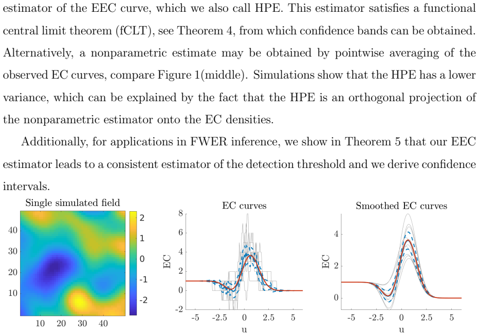
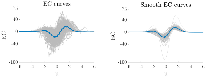
The central claim is that the Lipschitz-Killing curvatures are recoverable from a single observed Euler characteristic curve by linear projection: after pinning the curve by subtracting the known baseline $L_0\Phi^+$, the $d$-th LKC is estimated by $\hat L_d = (2\pi)^{d/2}/(d-1)! \int_{-\infty}^{\infty} H_{d-1}(u)\,\chi_f^\circ(u)\,du$. For Gaussian fields satisfying assumptions (G1)-(G4), this estimate is unbiased and has finite variance, and its sample average is consistent and asymptotically normal. For non-Gaussian fields satisfying a functional CLT, the bootstrap HPE applies the same projector to Gaussian multiplier fields generated from standardized residuals; the estimator equals the LKCs of the Gaussian field with the empirical correlation, and converges to the LKCs of the limiting field as the sample size grows. Plugging either LKC estimate into the Gaussian kinematic formula gives a smooth estimator of the EEC curve that inherits a functional CLT and yields confidence bands and consistent threshold estimates.
Load-bearing premise
The bootstrap estimator rests on the empirical correlation of the standardized residuals, and its derivatives up to order two, converging uniformly to the true correlation; if that convergence fails, the constructed Gaussian multiplier field does not have the right geometry and the LKC estimates no longer converge to the limiting field's LKCs.
Editorial extensions
If this is right
- LKC estimation no longer requires stationarity or isotropy: any domain where the Euler characteristic of excursion sets can be computed, including curved surfaces like the sphere or the cortical surface, becomes usable.
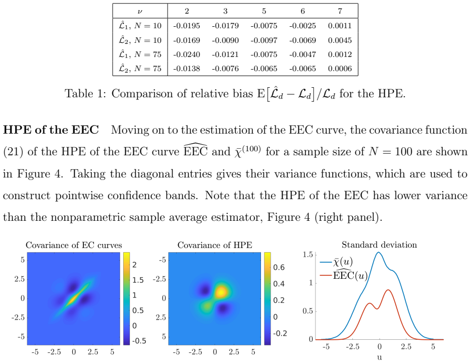
- The smooth HPE of the EEC curve is an orthogonal projection of the nonparametric average and has lower variance; the paper's functional CLT gives both pointwise and simultaneous confidence bands for the true EEC curve.
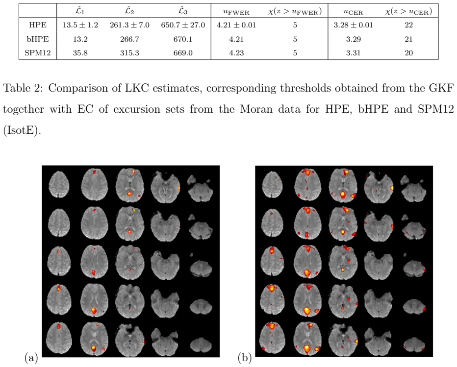
- The threshold solving $\widehat{\mathrm{EEC}}(u)=\alpha$ is a consistent estimator of the excursion threshold and is asymptotically Gaussian, so significance levels for fMRI activation maps and the expected number of false clusters can be reported with standard errors.
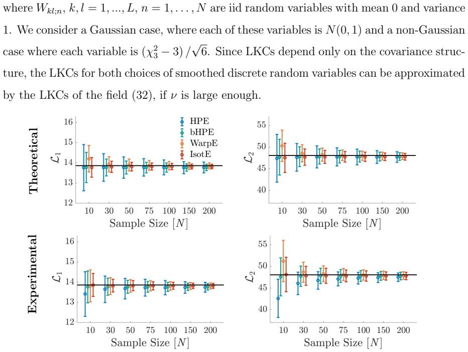
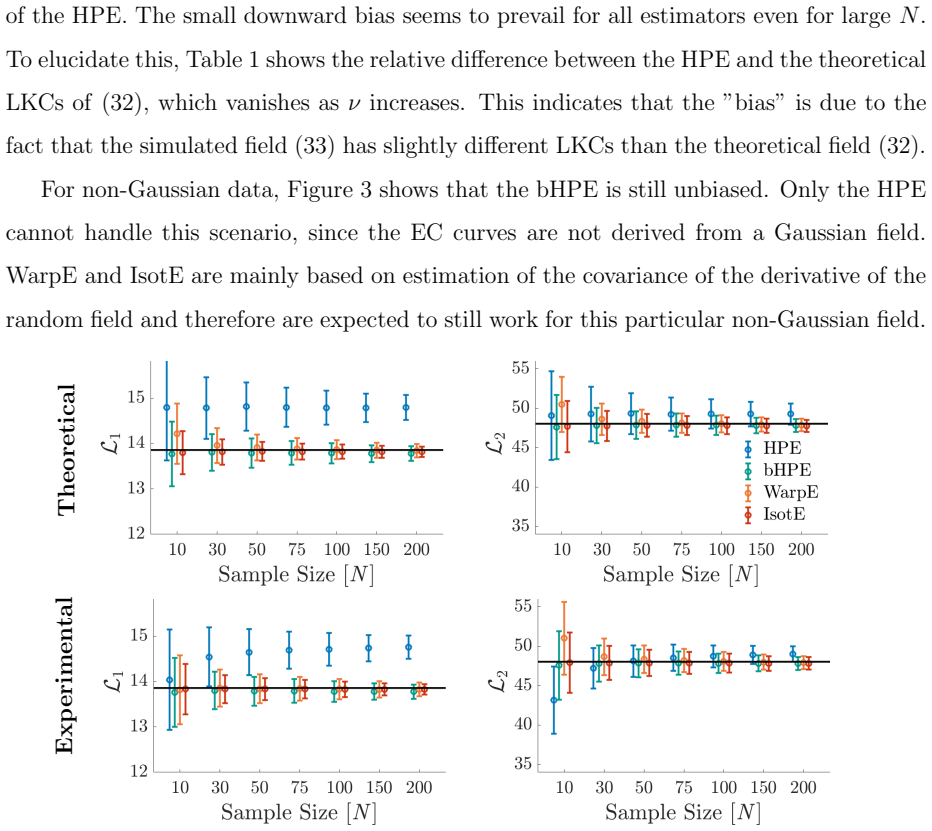
- For non-Gaussian observations, the bHPE estimates the LKCs of the Gaussian limiting field without knowing the field's mean or variance, extending the method to general linear models and standardized residual fields.
- In the cosmic microwave background example, the observed field's second LKC lies about 2.93 standard deviations from the mean of the simulations, giving a quantitative topological comparison between observed and simulated sky maps.
Reading between the lines
- The same projection structure should extend to Gaussian-related fields covered by the Gaussian kinematic formula, such as chi-squared and t fields, by replacing the EC densities with the corresponding Gaussian-related densities; the paper notes the extension for plug-in EEC estimators but does not develop the HPE there.
- The bHPE's consistency leans on uniform convergence of the empirical correlation and its derivatives, so in short samples the estimator is effectively estimating the LKCs of the empirical correlation; a practical diagnostic would be to compare bHPE outputs under different residual constructions on the same data.
- The critical-value representation of the HPE suggests an online or streaming implementation: an algorithm that passes through the field once and records critical values and topology changes yields the estimator without storing the entire field, connecting naturally to streaming Euler-curve algorithms.
- The CMB comparison points to a reusable diagnostic: comparing observed LKC estimates to simulation means can flag physical model mismatch, and the same logic could be applied to other cosmological maps to probe non-Gaussianity in the early universe.
Signed reviews
Editorial analysis
A structured set of objections, weighed in public.
Referee Report
Summary. The paper proposes Hermite projection estimators (HPE) for the Lipschitz-Killing curvatures (LKCs) of nonstationary smooth Gaussian random fields, based on projecting the observed Euler characteristic (EC) curve onto the EC densities in a weighted L2 space. A multiplier bootstrap variant (bHPE) is introduced to estimate the LKCs of the Gaussian limiting field of non-Gaussian or non-iid data. The paper proves unbiasedness, finite variance, consistency, and CLTs for the HPE and the resulting plug-in EEC estimator, derives asymptotic confidence bands, and analyzes the estimated detection threshold. The methods are evaluated on simulated 2D fields and applied to CMB and fMRI data. The main results are Theorems 1-5, with proofs in the appendix and code provided online.
Significance. If the results hold, this is a valuable contribution to random field theory and its applications in neuroimaging and cosmology. It offers a computationally simple, theoretically grounded alternative to stationarity-based LKC estimators, and the multiplier bootstrap extension to non-Gaussian limiting fields is novel and practically important. The paper ships reproducible code, includes extensive simulations comparing against existing methods, and gives concrete, falsifiable predictions (e.g., unbiasedness of the HPE under (G1)-(G4a), consistency of the bHPE under (R1)-(R2)). The proofs of Theorems 1, 2, 4, and 5 are largely rigorous, and the simulation results convincingly support the finite-sample claims. However, the proof of the central bHPE consistency theorem (Theorem 3(ii)) has a gap, and the theorem relies on an unverified regularity assumption about the Gaussian multiplier field, so the full consistency claim is not yet established.
major comments (3)
- [Section 3, Theorem 3(ii); Supplementary B.4] The proof of the convergence L(ˆr^{(N)}) → L(r) in Theorem 3(ii) requires convergence of the fourth-order mixed partial derivatives of the empirical correlation, because the Riemannian curvature tensor is expressed in B.4 in terms of E[∂d∂d' R_g^{(N)} ∂d''∂d''' R_g^{(N)}] = ∂^4_{s,s'} ˆr^{(N)}(s,s')|_{s=s'}. However, assumption (R2) only assumes uniform almost sure convergence of ˆr^{(N)} and its partial derivatives up to order 2. The sentence in B.4 asserting that this fourth-order quantity 'converges by (R2)' is therefore not justified. Since the LKC map is not, in general, a continuous function of only the second derivatives of the correlation, the convergence L(ˆr^{(N)}) → L(r) is an additional assumption rather than a consequence of (R2). This is a load-bearing gap for the main bHPE consistency claim. The authors should strengthen (R2) to include uniform convergence of derivatives up to order 4 (with appropriate domination) or prove continuity of the LKC functional under a weaker metric that only involves second derivatives.
- [Section 3, Theorem 3] The theorem assumes that, for almost all residuals R1,...,RN and all sufficiently large N, the Gaussian multiplier field R_g^{(N)} satisfies (G1)-(G4a). No sufficient conditions on the observed fields or residuals are provided under which this assumption holds. Since (G4) is itself admitted in Section 2 to be an active research topic, the bHPE consistency result is conditional on an unverified regularity property. The paper should either supply checkable conditions under which the GMF inherits (G1)-(G4a) from the residuals, or explicitly state Theorem 3 as a conditional result. As written, the abstract's claim that the bHPE 'allows estimation of LKCs ... of the limiting field' is stronger than what the theorem establishes.
- [Section 2, Corollary 1; Supplementary B.3] The proof of Corollary 1 infers superpolynomial decay of Cov[χf(u), χf(v)] from the finiteness of the double integrals in (10) for all d,d'. Finiteness of all polynomial moments of an integrable function does not by itself imply pointwise decay faster than every polynomial unless additional regularity (e.g., monotonicity or continuity of the covariance kernel in its tails) is assumed. This does not affect the main theorems, but as written the corollary's proof is incomplete. The authors should either prove the decay under explicit additional conditions or reformulate the corollary as a statement about polynomial moments of the covariance kernel.
minor comments (4)
- [Section 3, Theorem 3 statement] The phrase 'for almost all N > N′' is awkward because N is the fixed sample size in the theorem. It would be clearer to state 'for all N ≥ N0 almost surely' or 'for all sufficiently large N, almost surely over the residuals.'
- [Section 2, Theorem 2(ii)] In the statement 'the covariances σdd′ are finite for all d,d′ = 1,...,N', the upper limit N appears to be a typo and should be D, the dimension of the manifold.
- [Section 3, assumption (R2)] Assumption (R2) says that ˆr^{(N)}(s,s') and its partial derivatives up to order 2 converge uniformly, but the proof of Theorem 3(ii) uses fourth-order mixed partial derivatives. The notation should clarify whether derivatives are taken with respect to both arguments s and s', and the assumption should be stated in a form that makes the required order explicit.
- [Section 4, Theorem 4] Theorem 4 is stated 'under the assumptions (G1)-(G4)', but part (i) only requires that the arbitrary estimator ˆL^{(N)} be consistent and part (ii) only requires the CLT for ˆL^{(N)}. The hypotheses should be stated directly in terms of the estimator ˆL^{(N)} rather than referencing (G1)-(G4), which are conditions on the underlying field and not on the estimator.
Circularity Check
No circularity: the HPE and bHPE are plug-in/projection estimators whose theory rests on the externally cited Gaussian kinematic formula; the proof gap in Theorem 3 is a regularity issue, not a circular reduction.
full rationale
The central derivation is not circular. The HPE defines the LKCs as Hermite-projection coefficients of the EEC curve via the Gaussian kinematic formula (Eq. 6), and estimates them by applying the same linear functional to an observed EC curve (Eq. 9). This is a plug-in/method-of-moments estimator, not a fit: no parameter is adjusted to reproduce a target LKC, and unbiasedness follows from linearity plus the external GKF. The bHPE likewise uses Gaussian multiplier fields whose conditional correlation is the empirical correlation (Eq. 17), so the estimator is the plug-in L(rhat^(N)); consistency of plug-in requires continuity of the LKC map, which the paper attempts to show in B.4. The skeptical concern that B.4 implicitly needs fourth-order convergence of the empirical correlation while (R2) only supplies derivatives up to order 2 is a genuine correctness or assumption gap, not a circularity: the conclusion is not definitionally identical to the input. The self-citations in the paper (Telschow and Schwartzman 2019, Telschow et al. 2019) concern sufficient smoothness conditions and confidence-band constructions; they are not load-bearing for the main estimator identities and are not used to forbid alternatives. No equation in the paper reduces to its own input, and no fitted parameter is renamed as a prediction. Therefore the appropriate finding is no significant circularity, with the caveat that Theorem 3's consistency proof should be strengthened with an explicit fourth-order condition.
Assumptions & free parameters
assumptions (4)
- standard math Gaussian kinematic formula (GKF) expressing EEC as finite linear combination of EC densities with LKC coefficients.
- domain assumption The random field satisfies (G1)-(G4): mean zero, variance one, C^2 paths, nondegenerate derivative distribution, local Holder condition on second derivatives, and finite moments of the number of critical points.
- domain assumption Standardized residuals satisfy (R1) and (R2): vanishing sum, unit sum of squares, and uniform convergence of empirical correlation and its derivatives to the true correlation.
- ad hoc to paper The Gaussian multiplier field conditioned on residuals satisfies (G1)-(G4a) for almost all N.
Cite this review
Pith. "Pith review of Estimation of Expected Euler Characteristic Curves of Nonstationary Smooth Gaussian Random Fields." pith.science (2026). https://pith.science/paper/475AWMYL
@misc{pith2026190802493,
  author       = {Pith},
  title        = {Pith review of: Estimation of Expected Euler Characteristic Curves of Nonstationary Smooth Gaussian Random Fields},
  year         = {2026},
  howpublished = {\url{https://pith.science/paper/475AWMYL}},
  note         = {Machine review of arXiv:1908.02493}
}
read the original abstract
The expected Euler characteristic (EEC) curve of excursion sets of a Gaussian random field is used to approximate the distribution of its supremum for high thresholds. Viewed as a function of the excursion threshold, the EEC is expressed by the Gaussian kinematic formula (GKF) as a linear function of the Lipschitz-Killing curvatures (LKCs) of the field, which solely depend on the domain and covariance function of the field. So far its use for non-stationary Gaussian fields over non-trivial domains has been limited because in this case the LKCs are difficult to estimate. In this paper, consistent estimators of the LKCs are proposed as linear projections of "pinned" observed Euler characteristic curves and a linear parametric estimator of the EEC curve is obtained, which is more efficient than its nonparametric counterpart for repeated observations. A multiplier bootstrap modification reduces the variance of the estimator, and allows estimation of LKCs and EEC of the limiting field of non-Gaussian fields satisfying a functional CLT. The proposed methods are evaluated using simulations of 2D fields and illustrated in thresholding of 3D fMRI brain activation maps and cosmological simulations on the 2-sphere.
Figures
Figures from the paper (8 more)

Reference graph
Works this paper leans on
-
[1]
P. A. Ade, N. Aghanim, C. Armitage-Caplan, M. Arnaud, M. Ashdown, F. Atrio-Barandela, J. Aumont, C. Baccigalupi, A. J. Banday, R. Barreiro, et al. Planck 2013 results. xxiii. isotropy and statistics of the cmb. Astronomy & Astrophysics, 571: 0 A23, 2014
work page 2013
-
[2]
P. A. Ade, N. Aghanim, M. Arnaud, M. Ashdown, J. Aumont, C. Baccigalupi, A. Banday, R. Barreiro, J. Bartlett, N. Bartolo, et al. Planck 2015 results-xii. full focal plane simulations. Astronomy & Astrophysics, 594: 0 A12, 2016
work page 2015
-
[3]
R. J. Adler and J. E. Taylor. Random fields and geometry. Springer Science & Business Media, 2009
work page 2009
-
[4]
R. J. Adler, K. Bartz, S. C. Kou, and A. Monod. Estimating thresholding levels for random fields via euler characteristics. arXiv preprint arXiv:1704.08562, 2017
work page Pith review arXiv 2017
-
[5]
J.-M. Aza \" s and M. Wschebor. Level sets and extrema of random processes and fields. John Wiley & Sons, 2009
work page 2009
-
[6]
J. Bartlett, M. Bucher, J. Cardoso, G. Castex, J. Delabrouille, K. Ganga, Y. Giraud-H \'e raud, M. Le Jeune, G. Patanchon, M. Piat, et al. Planck 2015 results: Ix. diffuse component separation: Cmb maps. Astronomy and Astrophysics, 594: 0 A9--A9, 2016
work page 2015
-
[7]
E. T. Bullmore, J. Suckling, S. Overmeyer, S. Rabe-Hesketh, E. Taylor, and M. J. Brammer. Global, voxel, and cluster tests, by theory and permutation, for a difference between two groups of structural mr images of the brain. IEEE transactions on medical imaging, 18 0 (1): 0 32--42, 1999
work page 1999
-
[8]
D. Cheng and A. Schwartzman. Multiple testing of local maxima for detection of peaks in random fields. Annals of statistics, 45 0 (2): 0 529, 2017
work page 2017
Show all 34 references
-
[9]
Cheng, V
D. Cheng, V. Cammarota, Y. Fantaye, D. Marinucci, A. Schwartzman, et al. Multiple testing of local maxima for detection of peaks on the (celestial) sphere. Bernoulli, 26 0 (1): 0 31--60, 2020
2020
-
[10]
F. Eicker. Asymptotic normality and consistency of the least squares estimators for families of linear regressions. The Annals of Mathematical Statistics, pages 447--456, 1963
1963
-
[11]
Eklund, T
A. Eklund, T. E. Nichols, and H. Knutsson. Cluster failure: Why fmri inferences for spatial extent have inflated false-positive rates. Proceedings of the national academy of sciences, 113 0 (28): 0 7900--7905, 2016
2016
-
[12]
Estrade and J
A. Estrade and J. Fournier. Number of critical points of a gaussian random field: Condition for a finite variance. Statistics & Probability Letters, 118: 0 94--99, 2016
2016
-
[13]
K. M. Gorski, E. Hivon, A. J. Banday, B. D. Wandelt, F. K. Hansen, M. Reinecke, and M. Bartelmann. Healpix: A framework for high-resolution discretization and fast analysis of data distributed on the sphere. The Astrophysical Journal, 622 0 (2): 0 759, 2005
2005
-
[14]
J. R. Gott, A. L. Melott, and M. Dickinson. The sponge-like topology of large-scale structure in the universe. The Astrophysical Journal, 306: 0 341--357, 1986
1986
-
[15]
Heiss and H
T. Heiss and H. Wagner. Streaming algorithm for euler characteristic curves of multidimensional images. In International Conference on Computer Analysis of Images and Patterns, pages 397--409. Springer, 2017
2017
-
[16]
Hikage, Y
C. Hikage, Y. Suto, I. Kayo, A. Taruya, T. Matsubara, M. S. Vogeley, F. Hoyle, J. R. Gott III, J. Brinkmann, and S. collaboration. Three-dimensional genus statistics of galaxies in the sdss early data release. Publications of the Astronomical Society of Japan, 54 0 (5): 0 707-...
2002
-
[17]
S. J. Kiebel, J.-B. Poline, K. J. Friston, A. P. Holmes, and K. J. Worsley. Robust smoothness estimation in statistical parametric maps using standardized residuals from the general linear model. Neuroimage, 10 0 (6): 0 756--766, 1999
1999
-
[18]
Liebl and M
D. Liebl and M. Reimherr. Fast and fair simultaneous confidence bands for functional parameters. arXiv preprint arXiv:1910.00131, 2019
1910 arXiv
-
[19]
J. M. Moran, E. Jolly, and J. P. Mitchell. Social-cognitive deficits in normal aging. Journal of neuroscience, 32 0 (16): 0 5553--5561, 2012
2012
-
[20]
T. E. Nichols. Multiple testing corrections, nonparametric methods, and random field theory. Neuroimage, 62 0 (2): 0 811--815, 2012
2012
-
[21]
Pranav, H
P. Pranav, H. Edelsbrunner, R. Van de Weygaert, G. Vegter, M. Kerber, B. J. Jones, and M. Wintraecken. The topology of the cosmic web in terms of persistent betti numbers. Monthly Notices of the Royal Astronomical Society, 465 0 (4): 0 4281--4310, 2017
2017
-
[22]
Pranav, R
P. Pranav, R. J. Adler, T. Buchert, H. Edelsbrunner, B. J. Jones, A. Schwartzman, H. Wagner, and R. Van de Weygaert. Unexpected topology of the temperature fluctuations in the cosmic microwave background. Astronomy & Astrophysics, 627: 0 A163, 2019
2019
-
[23]
D. O. Siegmund and K. J. Worsley. Testing for a signal with unknown location and scale in a stationary gaussian random field. The Annals of Statistics, pages 608--639, 1995
1995
-
[24]
Sommerfeld, S
M. Sommerfeld, S. Sain, and A. Schwartzman. Confidence regions for spatial excursion sets from repeated random field observations, with an application to climate. Journal of the American Statistical Association, 113 0 (523): 0 1327--1340, 2018
2018
-
[25]
Taylor, A
J. Taylor, A. Takemura, R. J. Adler, et al. Validity of the expected euler characteristic heuristic. The Annals of Probability, 33 0 (4): 0 1362--1396, 2005
2005
-
[26]
J. E. Taylor and K. J. Worsley. Detecting sparse signals in random fields, with an application to brain mapping. Journal of the American Statistical Association, 102 0 (479): 0 913--928, 2007
2007
-
[27]
J. E. Taylor et al. A gaussian kinematic formula. The Annals of Probability, 34 0 (1): 0 122--158, 2006
2006
-
[28]
F. J. Telschow and A. Schwartzman. Simultaneous confidence bands for functional data using the gaussian kinematic formula. arXiv preprint arXiv:1901.06386, 2019
1901 arXiv
-
[29]
F. J. Telschow, M. R. Pierrynowski, and S. F. Huckemann. Confidence tubes for curves on so (3) and identification of subject-specific gait change after kneeling. arXiv preprint arXiv:1909.06583, 2019
1909 arXiv
-
[30]
A. W. Van der Vaart. Asymptotic statistics, volume 3. Cambridge university press, 2000
2000
-
[31]
K. J. Worsley. An unbiased estimator for the roughness of a multivariate Gaussian random field. Department of Mathematics and Statistics, McGill University Montr \'e al, Canada, 1996
1996
-
[32]
K. J. Worsley, A. C. Evans, S. Marrett, and P. Neelin. A three-dimensional statistical analysis for cbf activation studies in human brain. Journal of Cerebral Blood Flow & Metabolism, 12 0 (6): 0 900--918, 1992
1992
-
[33]
K. J. Worsley, S. Marrett, P. Neelin, A. C. Vandal, K. J. Friston, and A. C. Evans. A unified statistical approach for determining significant signals in images of cerebral activation. Human brain mapping, 4 0 (1): 0 58--73, 1996
1996
-
[34]
K. J. Worsley, J. E. Taylor, F. Tomaiuolo, and J. Lerch. Unified univariate and multivariate random field theory. Neuroimage, 23: 0 S189--S195, 2004
2004
Reviewed August 14, 2026 · model on record in the stance chip above.
Discussion (0). Continue with ORCID to comment.