REVIEW 6 major objections 5 minor 80 references
Noncooperative dynamics in election interference
T0 review · 6 major / 5 minor · reviewed 2026-08-14 · deepseek-v4-flash
Pith's one-line read If either player in an election-interference game treats the outcome as all-or-nothing, rational play drives both sides' interference spending up superexponentially as election day approaches.
desk verdict Worth engaging for the arms-race differential game result; the empirical 'captures' claim is in-sample and the tweet-proxy attribution is mismarked, but the theory deserves refereeing. read the letter →
The pith
A machine-rendered reading of the paper's core claim, the machinery that carries it, and where it could break.
The reading
What carries the argument
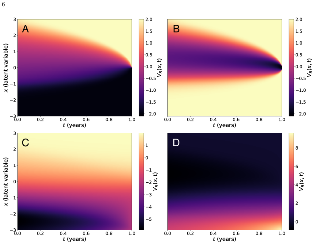
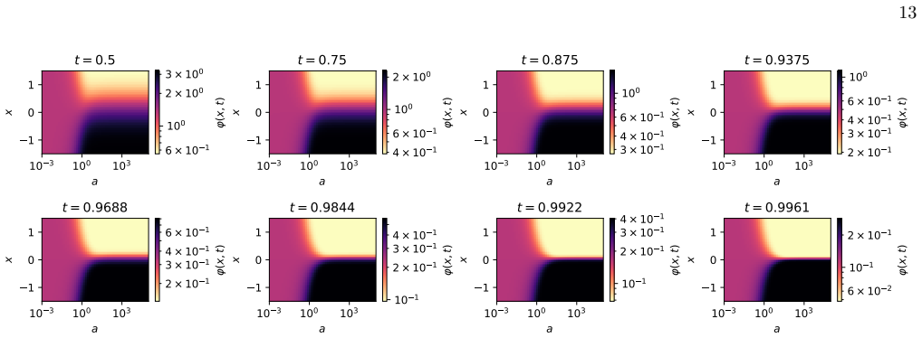
The load-bearing mechanism is the coupled Hamilton-Jacobi-Bellman system (Eqs. 11–12), a pair of nonlinear partial differential equations that describe each player's minimal expected cost as a function of time and the latent poll state. The Nash controls are the negative half-gradients of the value functions, and the quadratic running costs $u_i^2 - \lambda_i u_{\neg i}^2$ give the coupling through the opponent's effort. Discontinuous terminal payoffs, the Heaviside forms, make the terminal control behave like a Dirac mass, which is what drives the superexponential escalation. For the one-sided problem under a credible commitment by the opponent, a logarithmic change of variables linearizes the HJB equation into a backward Kolmogorov equation, and a Feynman-Kac path-integral representation supplies closed-form Laplace approximations for the value function and policy. The inferential apparatus is a Bayesian structural time series model with Gaussian random-walk priors on the latent controls, a logit-normal likelihood for the poll, and a normal likelihood for the normalized daily post counts.
What would settle it
Apply the same estimation pipeline to a second documented election-interference campaign with a hard-line payoff and daily activity data: if the inferred control magnitudes do not grow faster than exponentially in the final weeks before the election, the arms-race claim fails. A complementary check would be to compare the inferred control series against internal records of the operation, showing that post volume was uncorrelated with actual interference spending.
Extended reading notes
Core claim
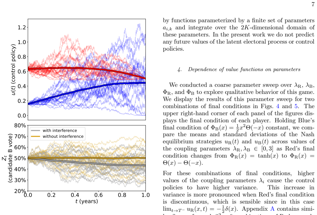
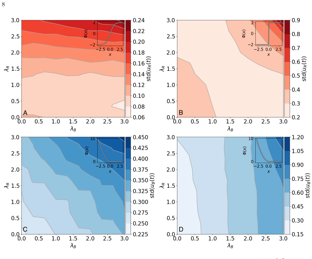
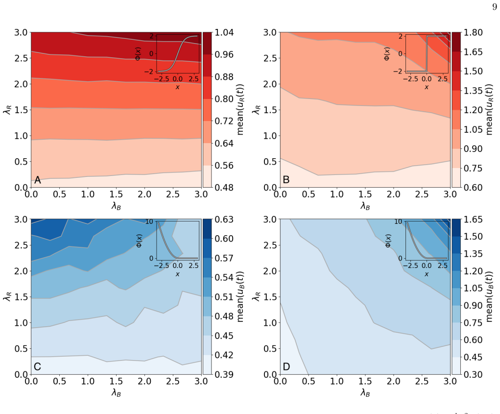
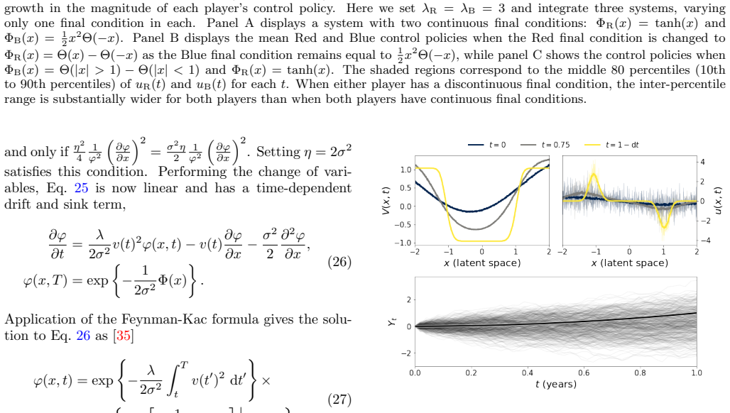
The central discovery is that the qualitative shape of the terminal payoff, not its scale, determines whether the game escalates. Red and Blue minimize cost functionals with quadratic running costs $u_i^2 - \lambda_i u_{\neg i}^2$ and terminal costs $\Phi_R(X_T)$ and $\Phi_B(X_T)$; the Nash equilibrium policies are $u_R(t)=-\tfrac12\partial V_R/\partial x$ and $u_B(t)=-\tfrac12\partial V_B/\partial x$, where the value functions solve a coupled pair of Hamilton-Jacobi-Bellman equations. Numerical sweeps over terminal conditions show that replacing a smooth payoff such as $\tanh(x)$ with a discontinuous Heaviside payoff such as $\Theta(x)-\Theta(-x)$ makes the value-function derivatives grow sharply near the terminal time, so both players' control magnitudes and their variances grow superexponentially. The paper's summary statement is that an all-or-nothing mindset by either Red or Blue about the final outcome leads to an arms race that negatively affects both players. In the empirical half, a Bayesian structural time series model infers latent controls and the latent poll from daily post counts and poll aggregates, and the theoretical model's free parameters are tuned to match those inferred series, giving an adequate fit over most of the campaign window.
Load-bearing premise
The empirical part of the paper rests on the premise that the daily count of posts from the flagged accounts measures Red's actual interference effort, so the inferred control series tracks real operations rather than an incidental feature of social-media activity.
Editorial extensions
If this is right
- If either side's terminal payoff is discontinuous, the equilibrium magnitudes and variances of both sides' interference controls grow superexponentially near the terminal time, so last-minute escalation should be the expected signature of the game.
- The 2016 fit implies that the observed surge in state-linked account activity is broadly consistent with an optimal control response once the race narrowed to two candidates, rather than with unstructured or random activity.
- A credible commitment by one side to a fixed strategy reduces the other side's problem to a single-player optimal-control problem with tractable approximations, so announced strategies can be converted into predictions about the opponent's counter-escalation.
- Because the arms-race property is stated for any strategic interaction of the form of Eqs. 3–5, the qualitative result should transfer to other contests with all-or-nothing final rewards, not only election interference.
Reading between the lines
- A sharper test of the arms-race mechanism would examine another documented interference campaign with a hard-line payoff: if inferred daily effort does not accelerate faster than exponential as the endpoint approaches, the mechanism is not universal.
- If the daily post series is read as a public signal rather than the true control, the fitted coupling parameters $\lambda_R,\lambda_B$ become interpretable as each side's sensitivity to the other's visible activity, a quantity that could be estimated for other geopolitical contests.
- The paper's acknowledged misfit in the first two weeks after the conventions suggests a natural extension: a higher-dimensional state that tracks several primary candidates and collapses when the field narrows, which would make the transition itself part of the game.
- The theory also implies that public social-media activity near an election is a strategic variable, so anomaly detection for influence operations should expect increased volume whenever a state publicly stakes its reputation on a candidate's victory.
Signed reviews
Editorial analysis
A structured set of objections, weighed in public.
Referee Report
Summary. The paper develops a continuous-time, two-player, nonzero-sum stochastic differential game of foreign election interference. A latent electoral process X_t is influenced by Red and Blue control policies u_R(t) and u_B(t), with quadratic running costs and a cross-player payoff parameter λ_i, and each player minimizes a terminal cost Φ_i(X_T). The authors derive coupled Hamilton-Jacobi-Bellman equations, solve them numerically for a variety of terminal payoff structures, and report that discontinuous, all-or-nothing terminal conditions lead to superexponential growth of both players' control magnitudes near the election. They also analyze a credible-commitment variant using path-integral and Laplace methods. The paper then confronts the model with 2016 U.S. presidential election polling data and tweet counts from the fivethirtyeight Russian troll dataset, using a Bayesian structural time series model to infer latent controls and then calibrating the game's parameters to those inferred quantities. The abstract claims that the analytical model 'adequately captures many temporal characteristics' of the election and social media activity.
Significance. The theoretical setup is clear, stylized, and potentially useful: the arms-race mechanism, if established rigorously, is a non-obvious qualitative insight about terminal payoff structure in strategic interference games. Strengths include a reproducible simulation codebase, explicit discussion of several model limitations, and analytic reductions for the credible-commitment case. However, the empirical contribution is currently an in-sample calibration rather than a predictive test, the Twitter proxy is attributed to the wrong type of actor, there is an unresolved sign inconsistency between the theory and the BSTS state equation, and two reported sets of fitted parameters disagree. These issues do not necessarily invalidate the theoretical core, but they substantially weaken the empirical claims made in the abstract and conclusions.
major comments (6)
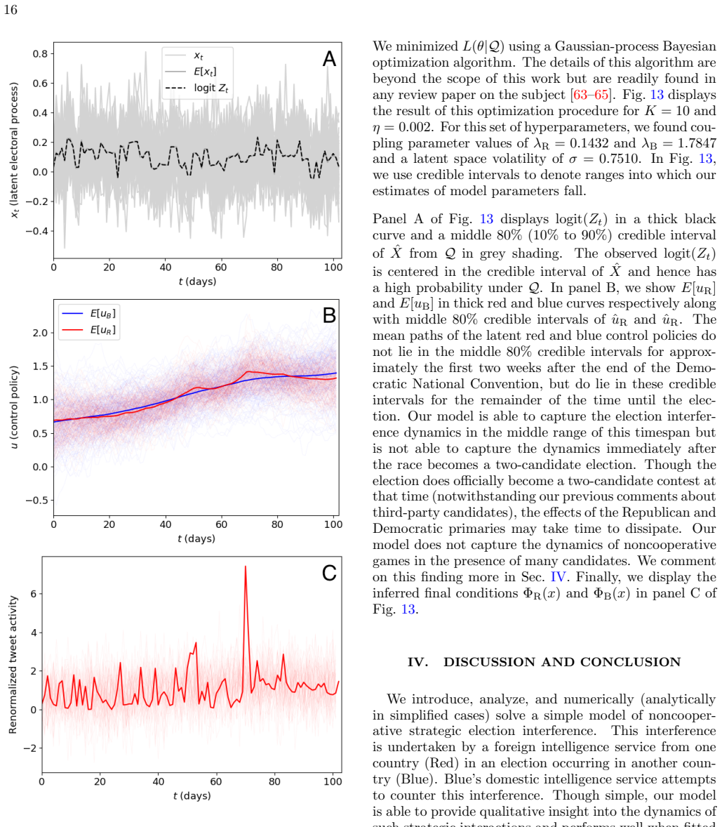
- [§II.B.3, §III, Eq. (49)] The empirical claim that Q 'adequately captures' the data is an in-sample calibration, not an independent test. The BSTS model M infers u_R, u_B, and X from the data using random-walk priors, and Q is then fit by minimizing the loss L(θ|Q) against M's posterior means, including the Legendre coefficients of the terminal payoff functions. The paper explicitly states in §II.B.3 that it does not predict any future values. Agreement between Q's credible intervals and M's inferred means is therefore partly produced by the fitting procedure and cannot serve as confirmation of the model. The section should be reframed as calibration or exploration, or supplemented with a genuine out-of-sample or posterior-predictive check.
- [§III, footnote [51]] The Twitter data are attributed to 'Russian military intelligence-associated' accounts and the empirical Red player is identified as 'the Russian military foreign intelligence service,' but the cited fivethirtyeight/russian-troll-tweets dataset consists of accounts associated with the Internet Research Agency, a private troll operation, not the GRU/SVR. Since tweet volume is the only direct observable for Red's control policy u_R, misidentifying the actor undermines the mapping from the data to the theoretical Red player. The attribution should be corrected and the implications of the actor mismatch for the empirical conclusions should be discussed.
- [§III, Eq. (46); §II.A, Eq. (3)] The BSTS state equation is inconsistent in sign with the theoretical state equation. The theory states dX_t = [u_R(t) + u_B(t)]dt + σ dW_t, while Eq. (46) gives X_t ~ N(X_{t-1} + u_{B,t-1} − u_{R,t-1}, 1). Combined with Eq. (48), where normalized tweet counts are modeled as N(u_R,t, σ_Tweets^2), and with Red's stated objective of favoring candidate A (Clinton), the inferred u_R has the opposite sign from the theoretical control policy unless an explicit reparameterization is introduced. This affects the sign and interpretation of the inferred controls and every fitted quantity that depends on them.
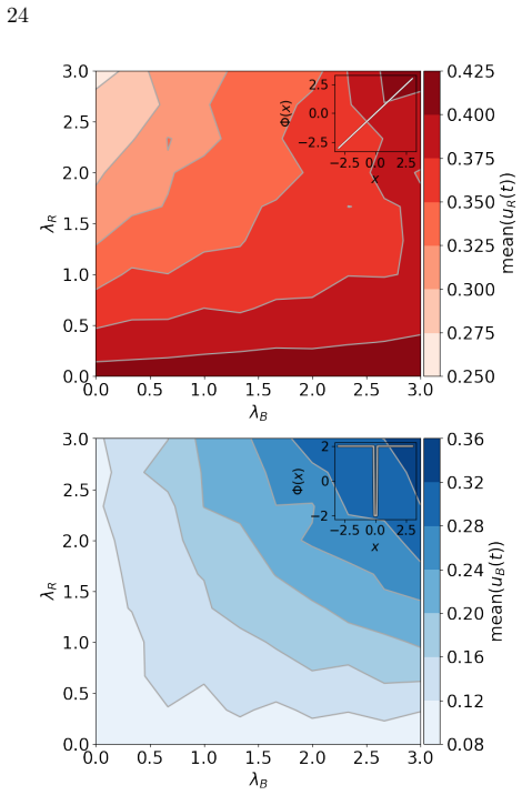
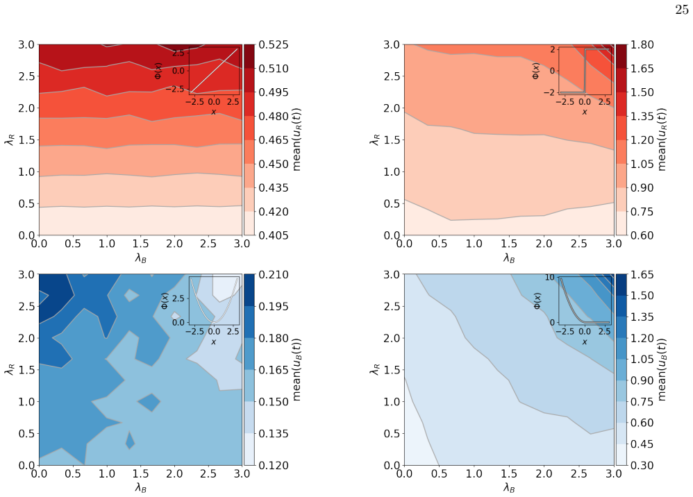
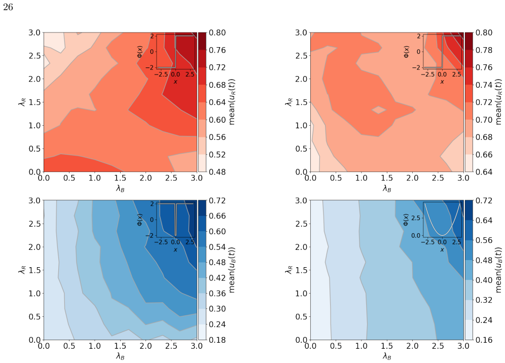
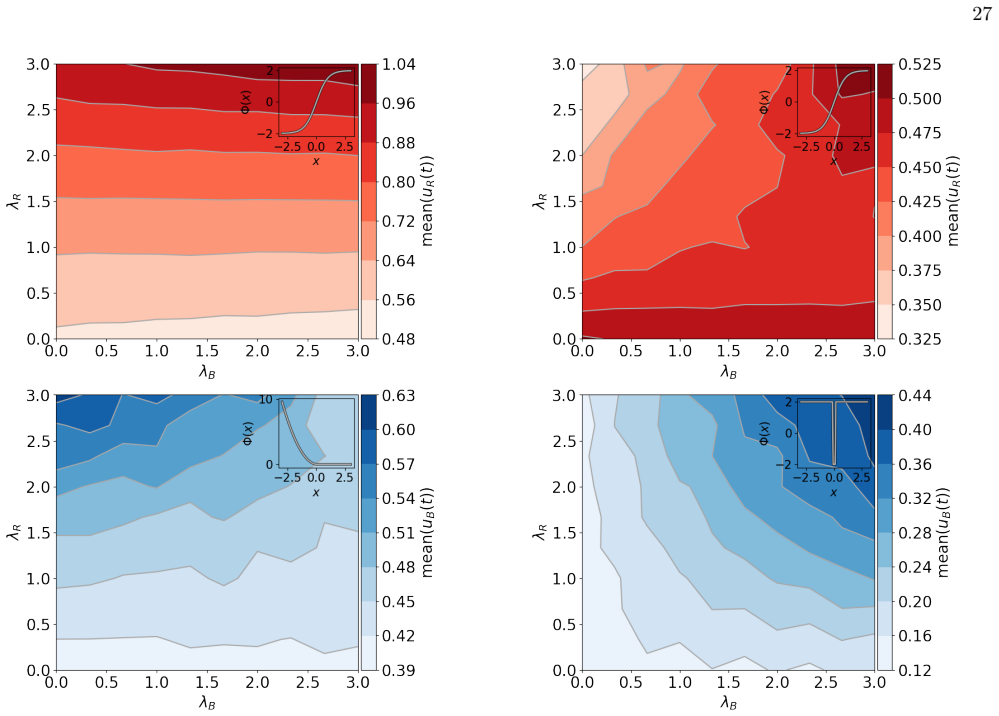
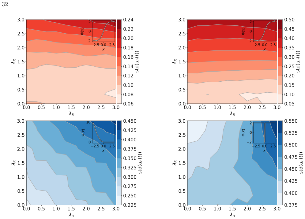
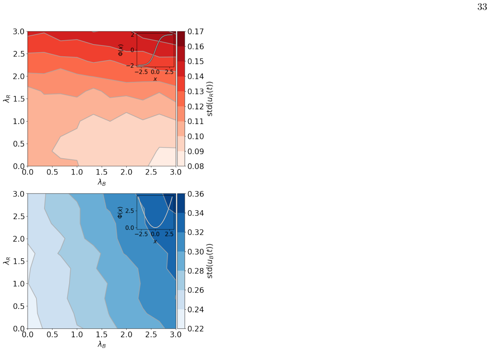
- [§II.B.4, Fig. 6] The statement that an all-or-nothing mindset by either player leads to an arms race is presented as a general feature, but the numerical evidence covers only selected terminal payoff functions and a single coupling value (λ_R = λ_B = 3) in Fig. 6, with nine combinations in Appendix A. Discontinuous terminal payoffs clearly produce steeper value-function gradients, but the specific claim of superexponential growth of both players' control magnitudes for arbitrary discontinuous final conditions requires either a proof or a systematic study over a wider class of terminal functions, parameters, and numerical resolutions before it is stated as a general result.
- [§III, Fig. 13] The reported fitted parameter values are internally inconsistent. The main text reports (λ_R, λ_B, σ) = (0.1432, 1.7847, 0.7510), while the caption of Fig. 13, for the same K = 10 and η = 0.002, reports (0.849, 0.727, 1.509). No explanation is given for the discrepancy, and it is unclear which parameter set was used to generate the displayed credible intervals. This needs to be reconciled before the empirical results can be assessed.
- [§II.B.3, Eqs. (11)–(12)] The inference and equilibrium analysis assume that the coupled HJB system has a unique solution for given final conditions Φ_R and Φ_B, and the manuscript admits that this uniqueness is not proved. Because the posterior in Eq. (21), the interpretation of the numerical solutions as subgame-perfect Nash equilibria, and the subsequent parameter inference all rely on this assumption, this is a load-bearing gap. A proof, a citation to a theorem covering this class of coupled systems, or an explicit statement that all equilibrium and inference results are contingent on uniqueness is needed.
minor comments (5)
- [Throughout] Several typographical errors remain, including 'foriegn' in §I, 'connvenience' in §II.A, and an unmatched parenthesis after 'Electoral College' in §II.A.
- [Footnote [30]] The Gaussian process citation contains an unresolved placeholder '[ ? ]' that must be completed before publication.
- [Fig. 13 caption] The caption's panel B description says 'middle 80% credible intervals of ˆu_R and ˆu_R'; this should presumably read 'of ˆu_R and ˆu_B.'
- [Eqs. (18)–(20)] The path-integral representation involving functional Gaussian distributions and the partition function Z is used only formally and is not used in the numerical solution; a brief statement clarifying that these expressions are not employed in the numerical work would reduce confusion.
- [§III, Eq. (48)] The tweet count series is normalized and shifted to have a minimum of zero and then modeled with a normal likelihood, discarding its count nature; a brief justification of this choice relative to the Poisson alternative mentioned in the text would be helpful.
Circularity Check
Empirical 'adequately captures' claim is an in-sample fit to the M-inferred latent controls that are then used as the validation target; the theoretical arms-race result is independent and not circular.
-
fitted input called prediction
[Section III (Application), Eq. 49 and Fig. 13; Discussion]
"After inferring the latent control policies and electoral process, we searched for the parameter values θ = (λR,λB,σ,ΦR,ΦB) of the theoretical model that best explain the observed data and inferred latent variables. ... The 𝓁2 terms in Eq. 49 penalize deviation by Q from the mean of M’s inferred posterior distribution."
The M-inferred posterior means of u_R, u_B, and X are simultaneously (i) the targets to which Q's parameters—including the Legendre-expanded final payoff functions Φ_R and Φ_B—are fitted by minimizing Eq. 49, and (ii) the benchmark against which Q's output is displayed in Fig. 13 and declared to 'capture' the election interference dynamics. The subsequent claim that 'the observed logit(Zt) is centered in the credible interval' and that the mean control paths 'do lie in these credible intervals' is therefore a report of the optimized loss, not an independent confirmation.
full rationale
The central theoretical result—that an all-or-nothing (discontinuous) terminal payoff for either player drives superexponential growth of both controls—follows from the coupled HJB equations (Eqs. 11-12) and is demonstrated numerically in Fig. 6; no fitted data enter that derivation, so that part of the paper is self-contained. The circularity is located in the empirical validation. The BSTS stage M constructs latent controls u_R and u_B with random-walk priors (Eqs. 44-45), identifies u_R almost directly with normalized tweet counts through Eq. 48, and has no direct observation of u_B. The theoretical model Q is then fit to M's posterior means by minimizing Eq. 49 over θ=(λ_R,λ_B,σ,Φ_R,Φ_B), and the same posterior means are used as the basis for the 'captures' verdict in Fig. 13. That is an in-sample calibration presented as confirmation, not a prediction. Consistent with this, the paper states it does not predict future values, and it provides no hold-out assessment. I also note a non-circularity issue: the main text reports (λ_R,λ_B,σ)=(0.1432,1.7847,0.7510) while the Fig. 13 caption reports (0.849,0.727,1.509) for the same K=10, η=0.002; this inconsistency is a correctness/reproducibility concern rather than a circularity. There are no load-bearing self-citations or imported uniqueness theorems. Overall: theoretical contribution independent (score would be low for that part), but the empirical adequacy claim is forced by construction, giving a partial circularity score of 6.
Assumptions & free parameters
free parameters (6)
- lambda_R (Red coupling parameter) =
0.1432 in main text; 0.849 in Fig. 13 caption (discrepancy)
- lambda_B (Blue coupling parameter) =
1.7847 in main text; 0.727 in Fig. 13 caption (discrepancy)
- sigma (latent volatility) =
0.7510 in main text; 1.509 in Fig. 13 caption (discrepancy)
- Legendre coefficients a_{R,k}, a_{B,k}, k=0..10 =
not individually reported; 21 values fitted
- K (Legendre truncation order) =
10
- eta (loss regularization) =
0.002
assumptions (6)
- ad hoc to paper Coupled HJB system (Eqs. 11 and 12) has a unique solution for given final conditions Phi_R and Phi_B.
- domain assumption The latent election process has zero endogenous drift; controls enter additively and affect only the mean, not volatility.
- domain assumption Running costs reduce to u_i^2 - lambda_i u_neg_i^2 by Taylor expansion under even-function and zero-cost-at-zero assumptions.
- standard math Feynman-Kac and path integral control formulas apply to the transformed HJB equation (Eq. 26).
- domain assumption Tweet volume, after normalization, is a noisy observation of Red's control u_R.
- ad hoc to paper The BSTS state equation uses -u_R where the theory uses +u_R; this is either a sign reparameterization or a model inconsistency.
invented entities (3)
-
Latent electoral process X_t
independent evidence
-
Latent Red control policy u_R(t)
independent evidence
-
Latent Blue control policy u_B(t)
Cite this review
Pith. "Pith review of Noncooperative dynamics in election interference." pith.science (2026). https://pith.science/paper/ZLBN5H5O
@misc{pith2026190802793,
  author       = {Pith},
  title        = {Pith review of: Noncooperative dynamics in election interference},
  year         = {2026},
  howpublished = {\url{https://pith.science/paper/ZLBN5H5O}},
  note         = {Machine review of arXiv:1908.02793}
}
read the original abstract
Foreign power interference in domestic elections is an existential threat to societies. Manifested through myriad methods from war to words, such interference is a timely example of strategic interaction between economic and political agents. We model this interaction between rational game players as a continuous-time differential game, constructing an analytical model of this competition with a variety of payoff structures. All-or-nothing attitudes by only one player regarding the outcome of the game lead to an arms race in which both countries spend increasing amounts on interference and counter-interference operations. We then confront our model with data pertaining to the Russian interference in the 2016 United States presidential election contest. We introduce and estimate a Bayesian structural time series model of election polls and social media posts by Russian Twitter troll accounts. Our analytical model, while purposefully abstract and simple, adequately captures many temporal characteristics of the election and social media activity. We close with a discussion of our model's shortcomings and suggestions for future research.
Figures

Figures from the paper (23 more)








Reference graph
Works this paper leans on
-
[1]
Choice of final conditions Finding optimal play in noncooperative games often requires solving the game backward through time [23–26]. Therefore, we must define final conditions that specify the cost that Red and Blue incur from the actual election result φ(XT ). Red and Blue might have different final conditions because of their qualitatively distinct objec- ...
-
[2]
Value functions Applying the dynamic programming principle [17, 18] to Eqs. 3, 4, and 5 leads to a system of coupled Hamilton- Jacobi-Bellman equations for the Red and Blue value functions, −∂VR ∂t = min uR {∂VR ∂x [uR +uB] +u2 R−λRu2 B + σ2 2 ∂2VR ∂x2 } , (7) and −∂VB ∂t = min uB {∂VB ∂x [uR +uB] +u2 B−λBu2 R + σ2 2 ∂2VB ∂x2 } . (8) The dynamic programmi...
-
[3]
We plot the control policies in the top panel
For this example, we simulate the game with param- eters λR =λB = 2, ΦR(x) =x, and Φ B(x) = 1 2x2Θ(−x). We plot the control policies in the top panel. The mean control policies E[uR] and E[uB] are displayed in thicker curves. For this parameter set, it is optimal for Red to begin play with a larger amount of interference than Blue does and on average decr...
-
[4]
11 and 12 are functions of the final conditions VR(x,T ) = Φ R(x) and VB(x,T ) = ΦB(x)
Inference and prediction The solutions to Eqs. 11 and 12 are functions of the final conditions VR(x,T ) = Φ R(x) and VB(x,T ) = ΦB(x). It is possible to perform both inference and pre- diction at times t < Teven when Φ R(x) and Φ B(x) are not known. To do this, we assume that the system given by Eqs. 11 and 12 has a unique solution given particular final co...
-
[5]
Dependence of value functions on parameters We conducted a coarse parameter sweep over λR, λB, ΦR, and ΦB to explore qualitative behavior of this game. We display the results of this parameter sweep for two combinations of final conditions in Figs. 4 and 5. The upper right-hand corner of each panel of the figures dis- plays the final condition of each player...
-
[6]
The BKE can be solved using path integral methods [34]
Path integral control Though nonlinear, this HJB equation can be trans- formed into a backward Kolmogorov equation (BKE) through a change of variables. The BKE can be solved using path integral methods [34]. Setting V (x,t ) = −η logϕ(x,t ), substituting in Eq. 25, and performing the differentiation, we are able to remove the nonlinearity if 10 FIG. 6. In ...
-
[7]
Dependence on a free parameter The Laplace-approximated value function may depend on a free parameter a that can be used as a “control knob” to adjust the approximation. For example, player i might usea to tune the sensitivity of the approximation to the electoral process’s distance from a dead-heat. Ide- ally, the approximated control policy should have ...
-
[8]
On the importance of elections and ideology for government pol- icy in a multi-party system
Paul SA Renaud and Frans AAM van Winden. On the importance of elections and ideology for government pol- icy in a multi-party system. In The Logic of Multiparty Systems, pages 191–207. Springer, 1987
work page 1987
Show all 80 references
-
[9]
What makes elections free and fair? Journal of Democracy, 8(3):32–46, 1997
Jorgen Elklit and Palle Svensson. What makes elections free and fair? Journal of Democracy, 8(3):32–46, 1997
1997
-
[10]
When the great power gets a vote: The effects of great power electoral interventions on election results
Dov H Levin. When the great power gets a vote: The effects of great power electoral interventions on election results. International Studies Quarterly , 60(2):189–202, 2016
2016
-
[11]
The legitimacy of foreign intervention in elections: The ukrainian response
Stephen Shulman and Stephen Bloom. The legitimacy of foreign intervention in elections: The ukrainian response. Review of International Studies , 38(2):445–471, 2012
2012
-
[12]
Taking sides in other peoples elections: The polarizing effect of for- eign intervention
Daniel Corstange and Nikolay Marinov. Taking sides in other peoples elections: The polarizing effect of for- eign intervention. American Journal of Political Science, 56(3):655–670, 2012
2012
-
[13]
Partisan electoral interventions by the great powers: Introducing the PEIG Dataset
Dov H Levin. Partisan electoral interventions by the great powers: Introducing the PEIG Dataset. Conflict Management and Peace Science , 36(1):88–106, 2019
2019
-
[14]
Confidence Building Measures for the Cyber Domain
Erica D Borghard and Shawn W Lonergan. Confidence Building Measures for the Cyber Domain. Strategic Stud- ies Quarterly, 12(3):10–49, 2018
2018
-
[15]
Voting for Trouble? Partisan Electoral Interventions and Domestic Terrorism
Dov H Levin. Voting for Trouble? Partisan Electoral Interventions and Domestic Terrorism. Terrorism and Political Violence, pages 1–17, 2018
2018
-
[16]
Doxing democracy: influencing elections via cyber voter interference
Isabella Hansen and Darren J Lim. Doxing democracy: influencing elections via cyber voter interference. Con- temporary Politics, 25(2):150–171, 2019
2019
-
[17]
Why Do States Intervene in the Elections of Others? Available at SSRN 3435138 , 2019
Johannes Bubeck, Kai J¨ ager, Nikolay Marinov, and Fed- erico Nanni. Why Do States Intervene in the Elections of Others? Available at SSRN 3435138 , 2019
2019
-
[18]
New York Times, Apr 2019
Read the Mueller Report: Searchable Document and Index: https://www.nytimes.com/interactive /2019/04/18/us/politics/mueller-report-document.html. New York Times, Apr 2019
2019
-
[19]
Trends and random walks in macroeconmic time series: some evi- dence and implications
Charles R Nelson and Charles R Plosser. Trends and random walks in macroeconmic time series: some evi- dence and implications. Journal of monetary economics , 10(2):139–162, 1982
1982
-
[20]
Integration versus trend sta- tionary in time series
David N DeJong, John C Nankervis, N Eugene Savin, and Charles H Whiteman. Integration versus trend sta- tionary in time series. Econometrica: Journal of the Econometric Society, pages 423–433, 1992
1992
-
[21]
Handbook of Stochastic Methods , volume 3
Crispin W Gardiner. Handbook of Stochastic Methods , volume 3. Springer Berlin, 1985. 21
1985
-
[22]
Dynamical systems: a unified colored-noise approximation
Peter Jung and Peter H¨ anggi. Dynamical systems: a unified colored-noise approximation. Physical Review A, 35(10):4464, 1987
1987
-
[23]
Colored noise in dynami- cal systems
Peter H¨ anggi and Peter Jung. Colored noise in dynami- cal systems. Advances in Chemical Physics , 89:239–326, 1995
1995
-
[24]
Dynamic programming and a new for- malism in the calculus of variations
Richard Bellman. Dynamic programming and a new for- malism in the calculus of variations. Proceedings of the National Academy of Sciences of the United States of America, 40(4):231, 1954
1954
-
[25]
Dynamic programming
Richard Bellman. Dynamic programming. Science, 153(3731):34–37, 1966
1966
-
[26]
Reinforcement learning: An introduction
Richard S Sutton and Andrew G Barto. Reinforcement learning: An introduction. MIT press, 2018
2018
-
[27]
An introduction to stochastic control theory, path integrals and reinforcement learning
Hilbert J Kappen. An introduction to stochastic control theory, path integrals and reinforcement learning. InAIP conference proceedings, volume 887, pages 149–181. AIP, 2007
2007
-
[28]
Courier Corporation, 2012
Karl J ˚Astr¨ om.Introduction to stochastic control theory. Courier Corporation, 2012
2012
-
[29]
The separa- tion principle in stochastic control, redux
Tryphon T Georgiou and Anders Lindquist. The separa- tion principle in stochastic control, redux. IEEE Trans- actions on Automatic Control , 58(10):2481–2494, 2013
2013
-
[30]
¨Uber eine anwendung der mengenlehre auf die theorie des schachspiels
Ernst Zermelo. ¨Uber eine anwendung der mengenlehre auf die theorie des schachspiels. In Proceedings of the fifth international congress of mathematicians , volume 2, pages 501–504. Cambridge University Press Cambridge, UK, 1913
1913
-
[31]
Non-cooperative games
John Nash. Non-cooperative games. Annals of mathe- matics, pages 286–295, 1951
1951
-
[32]
Noncooperative game theory for industrial organization: an introduction and overview
Drew Fudenberg and Jean Tirole. Noncooperative game theory for industrial organization: an introduction and overview. Handbook of industrial Organization , 1:259– 327, 1989
1989
-
[33]
Microeconomic theory, volume 1
Andreu Mas-Colell, Michael Dennis Whinston, Jerry R Green, et al. Microeconomic theory, volume 1. Oxford university press New York, 1995
1995
-
[34]
Stochastic differen- tial games and viscosity solutions of Hamilton–Jacobi– Bellman–Isaacs equations
Rainer Buckdahn and Juan Li. Stochastic differen- tial games and viscosity solutions of Hamilton–Jacobi– Bellman–Isaacs equations. SIAM Journal on Control and Optimization, 47(1):444–475, 2008
2008
-
[35]
Two person zero-sum game in weak formulation and path dependent Bellman– Isaacs equation
Triet Pham and Jianfeng Zhang. Two person zero-sum game in weak formulation and path dependent Bellman– Isaacs equation. SIAM Journal on Control and Optimiza- tion, 52(4):2090–2121, 2014
2014
-
[36]
Code to recreate simulations and plots in this paper, or to create new simulations and “what-if” scenarios, is located at https://gitlab.com/daviddewhurst/red-blue-game
-
[37]
Here is an example of this type of approximation
There is a large literature on nonparametric functional approximation that we cannot review here. Here is an example of this type of approximation. If {xk}1≤k≤K is any partition of [ a,b ) and the vector (Φ R(xk), ΦB(xk)) were jointly distributed Gaussian on R2K, then we say t...
-
[38]
Monte carlo esti- mation of bayesian credible and hpd intervals
Ming-Hui Chen and Qi-Man Shao. Monte carlo esti- mation of bayesian credible and hpd intervals. Journal of Computational and Graphical Statistics , 8(1):69–92, 1999
1999
-
[39]
C3: nuclear command, control coop- eration
Valery E Yarynich. C3: nuclear command, control coop- eration. Center for Defense Information, 2003
2003
-
[40]
False alarms, true dangers? RAND Corporation document PE-191-TSF, DOI , 10, 2016
Anthony M Barrett. False alarms, true dangers? RAND Corporation document PE-191-TSF, DOI , 10, 2016
2016
-
[41]
Path integrals and symmetry breaking for optimal control theory
Hilbert J Kappen. Path integrals and symmetry breaking for optimal control theory. Journal of Statistical Mechan- ics: Theory and Experiment , 2005(11):P11011, 2005
2005
-
[42]
On distributions of certain Wiener function- als
Mark Kac. On distributions of certain Wiener function- als. Transactions of the American Mathematical Society, 65(1):1–13, 1949
1949
-
[43]
Weak-noise limit of a piecewise-smooth stochastic differential equation
Yaming Chen, Adrian Baule, Hugo Touchette, and Wol- fram Just. Weak-noise limit of a piecewise-smooth stochastic differential equation. Physical Review E , 88(5):052103, 2013
2013
-
[44]
Per- sistence of saddle behavior in the nonsmooth limit of smooth dynamical systems
Julie Leifeld, Kaitlin Hill, and Andrew Roberts. Per- sistence of saddle behavior in the nonsmooth limit of smooth dynamical systems. arXiv preprint arX- iv:1504.04671, 2015
2015 arXiv
-
[45]
Asymptotic derivation of Langevin- like equation with non-gaussian noise and its analyti- cal solution
Kiyoshi Kanazawa, Tomohiko G Sano, Takahiro Sagawa, and Hisao Hayakawa. Asymptotic derivation of Langevin- like equation with non-gaussian noise and its analyti- cal solution. Journal of Statistical Physics , 160(5):1294– 1335, 2015
2015
-
[46]
Inferring parameters of prey switching in a 1 predator–2 prey plankton system with a linear pref- erence tradeoff
Sofia H Piltz, Lauri Harhanen, Mason A Porter, and Philip K Maini. Inferring parameters of prey switching in a 1 predator–2 prey plankton system with a linear pref- erence tradeoff. Journal of Theoretical Biology, 456:108– 122, 2018
2018
-
[47]
The Invisible Front: Russia, Trolls, and the Information War against Ukraine
Peter Tanchak. The Invisible Front: Russia, Trolls, and the Information War against Ukraine. Revolution and War in Contemporary Ukraine: The Challenge of Change, 161:253, 2017
2017
-
[48]
Troll factories: The internet research agency and state-sponsored agenda building
Brandon C Boatwright, Darren L Linvill, and Patrick L Warren. Troll factories: The internet research agency and state-sponsored agenda building. Resource Centre on Media Freedom in Europe, 2018
2018
-
[49]
Analyzing the digital traces of political manipulation: the 2016 Russian interference Twitter campaign
Adam Badawy, Emilio Ferrara, and Kristina Lerman. Analyzing the digital traces of political manipulation: the 2016 Russian interference Twitter campaign. In 2018 IEEE/ACM International Conference on Advances in Social Networks Analysis and Mining (ASONAM) , pages 258–265. IEEE, 2018
2016
-
[50]
Characterizing the Internet Research Agen- cys Social Media Operations During the 2016 US Presi- dential Election using Linguistic Analyses
Ryan L Boyd, Alexander Spangher, Adam Fourney, Besmira Nushi, Gireeja Ranade, James Pennebaker, and Eric Horvitz. Characterizing the Internet Research Agen- cys Social Media Operations During the 2016 US Presi- dential Election using Linguistic Analyses. 2018
2016
-
[51]
Internet Research Agency Twitter activity predicted 2016 US election polls
Damian J Ruck, Natalie M Rice, Joshua Borycz, and R Alexander Bentley. Internet Research Agency Twitter activity predicted 2016 US election polls. First Monday, 24(7), 2019
2016
-
[52]
Detecting influence campaigns in social networks using the Ising model
Nicolas Guenon des Mesnards and Tauhid Zaman. Detecting influence campaigns in social networks using the Ising model. arXiv preprint arXiv:1805.10244 , 2018
2018 arXiv
-
[53]
Still out there: Modeling and Identifying Russian Troll Accounts on Twitter
Jane Im, Eshwar Chandrasekharan, Jackson Sargent, Paige Lighthammer, Taylor Denby, Ankit Bhargava, Lib- by Hemphill, David Jurgens, and Eric Gilbert. Still out there: Modeling and Identifying Russian Troll Accounts on Twitter. arXiv preprint arXiv:1901.11162 , 2019
1901 arXiv
-
[54]
Forecasting elections using compartmental models of infections
Alexandria Volkening, Daniel F Linder, Mason A Porter, and Grzegorz A Rempala. Forecasting elections using compartmental models of infections. arXiv preprint arX- 22 iv:1811.01831, 2018
2018 arXiv
-
[55]
Forecasting elections: Comparing pre- diction markets, polls, and their biases
David Rothschild. Forecasting elections: Comparing pre- diction markets, polls, and their biases. Public Opinion Quarterly, 73(5):895–916, 2009
2009
-
[56]
Dynamic Bayesian forecasting of presi- dential elections in the states
Drew A Linzer. Dynamic Bayesian forecasting of presi- dential elections in the states. Journal of the American Statistical Association, 108(501):124–134, 2013
2013
-
[57]
Forecasting elections with non-representative polls
Wei Wang, David Rothschild, Sharad Goel, and Andrew Gelman. Forecasting elections with non-representative polls. International Journal of Forecasting , 31(3):980– 991, 2015
2015
-
[58]
Data can be downloaded at https://github.com/ fivethirtyeight/russian-troll-tweets/
-
[59]
Pollsters struggle to explain failures of us presidential forecasts
Ramin Skibba. Pollsters struggle to explain failures of us presidential forecasts. Nature News, 539(7629):339, 2016
2016
-
[60]
Constrained by duality: Third- party master narratives in the 2016 presidential election
Ryan Neville-Shepard. Constrained by duality: Third- party master narratives in the 2016 presidential election. American Behavioral Scientist, 61(4):414–427, 2017
2016
-
[61]
realclearpolitics.com/epolls/2016/president/ us/general_election_trump_vs_clinton_vs_johnson_ vs_stein-5952.html
Data can be downloaded at https://www. realclearpolitics.com/epolls/2016/president/ us/general_election_trump_vs_clinton_vs_johnson_ vs_stein-5952.html
2016
-
[62]
Bayesian Time Series Models
David Barber, A Taylan Cemgil, and Silvia Chiappa. Bayesian Time Series Models . Cambridge University Press, 2011
2011
-
[63]
Sandsynlighedsregning og telefon- samtaler
Agner Krarup Erlang. Sandsynlighedsregning og telefon- samtaler. Nyt tidsskrift for Matematik , 20:33–39, 1909
1909
-
[64]
The poisson process as a model for a diver- sity of behavioral phenomena
Georg Rasch. The poisson process as a model for a diver- sity of behavioral phenomena. In International congress of psychology, volume 2, page 2, 1963
1963
-
[65]
Regression models and life-tables
David R Cox. Regression models and life-tables. Journal of the Royal Statistical Society: Series B (Methodologi- cal), 34(2):187–202, 1972
1972
-
[66]
Point processes, volume 12
David Roxbee Cox and Valerie Isham. Point processes, volume 12. CRC Press, 1980
1980
-
[67]
The No- U-Turn sampler: adaptively setting path lengths in Hamiltonian Monte Carlo
Matthew D Hoffman and Andrew Gelman. The No- U-Turn sampler: adaptively setting path lengths in Hamiltonian Monte Carlo. Journal of Machine Learn- ing Research, 15(1):1593–1623, 2014
2014
-
[68]
Inference from iterative simulation using multiple sequences
Andrew Gelman, Donald B Rubin, et al. Inference from iterative simulation using multiple sequences. Statistical Science, 7(4):457–472, 1992
1992
-
[69]
General methods for monitoring convergence of iterative simula- tions
Stephen P Brooks and Andrew Gelman. General methods for monitoring convergence of iterative simula- tions. Journal of Computational and Graphical Statistics, 7(4):434–455, 1998
1998
-
[70]
A tutorial on Bayesian optimization of expensive cost func- tions, with application to active user modeling and hier- archical reinforcement learning
Eric Brochu, Vlad M Cora, and Nando De Freitas. A tutorial on Bayesian optimization of expensive cost func- tions, with application to active user modeling and hier- archical reinforcement learning. arXiv preprint arX- iv:1012.2599, 2010
2010 arXiv
-
[71]
Taking the human out of the loop: A review of Bayesian optimization
Bobak Shahriari, Kevin Swersky, Ziyu Wang, Ryan P Adams, and Nando De Freitas. Taking the human out of the loop: A review of Bayesian optimization. Proceedings of the IEEE , 104(1):148–175, 2015
2015
-
[72]
A tutorial on bayesian optimization.arX- iv preprint arXiv:1807.02811 , 2018
Peter I Frazier. A tutorial on bayesian optimization.arX- iv preprint arXiv:1807.02811 , 2018
2018 arXiv
-
[73]
Election predictions as martin- gales: An arbitrage approach
Nassim Nicholas Taleb. Election predictions as martin- gales: An arbitrage approach. Quantitative Finance , 18(1):1–5, 2018
2018
-
[74]
Using the HJB integrator red blue pdes.py included in the code at https://gitlab.com/daviddewhurst/ red-blue-game, the reader may further investigate the effects of changes in the drift and running cost terms on the qualitative nature of solutions to the coupled HJB system
-
[75]
Stochastic variational inference
Matthew D Hoffman, David M Blei, Chong Wang, and John Paisley. Stochastic variational inference. The Journal of Machine Learning Research, 14(1):1303–1347, 2013
2013
-
[76]
Varia- tional inference with normalizing flows
Danilo Jimenez Rezende and Shakir Mohamed. Varia- tional inference with normalizing flows. arXiv preprint arXiv:1505.05770, 2015
2015 arXiv
-
[77]
Variational inference: A review for statisticians
David M Blei, Alp Kucukelbir, and Jon D McAuliffe. Variational inference: A review for statisticians. Journal of the American statistical Association , 112(518):859– 877, 2017
2017
-
[78]
Advances in variational inference
Cheng Zhang, Judith Butepage, Hedvig Kjellstrom, and Stephan Mandt. Advances in variational inference. IEEE transactions on pattern analysis and machine intelli- gence, 2018. 23 Appendix A: Coupling parameter sweeps We conducted parameter sweeps over different values of the cou...
2018
-
[79]
11 and 12
Expected value of ui(t) We display the mean paths of draws from the distri- butions of control policies generated by solutions to Eqs. 11 and 12. FIG. 16. Parameter sweep over coupling parameters λR,λ B with Red final condition Φ R(x) = x and Blue final condition ΦB(x) = 1 2x2Θ(...
-
[80]
11 and 12
Standard deviation of ui(t) We display the standard deviation of draws from the distributions of control policies generated by solutions to Eqs. 11 and 12. FIG. 25. Parameter sweep over coupling parameters λR,λ B with Red final condition Φ R(x) = x and Blue final condition ΦB(x)...
Reviewed August 14, 2026 · model on record in the stance chip above.
Discussion (0). Continue with ORCID to comment.